TOC
Background
This project came about during Hack for Sweden 2019. Our team was busy trying to develop an idea for allowing people to get external validation for their skill sets, for finding jobs. One of the parts of this project was that we wanted to make it possible to decide which skills would improve one’s employability to the greatest extent. In Sweden, there are several excellent resources for doing this.
My idea was to be able to search for one or more skills, and then see which other skills were most likely to co-occur in the same adverts. To give an example: imagine someone were to be a painter. We would want to figure out what other things they should work on in order to maximise their employability.
To operationalise this idea, we want to select those adverts which contained one or more terms, and then see which other terms occur most often in those adverts. This sounded like a really easy task, but it turned out to be more difficult than imagined with such a large dataset, and gave me a really great opportunity to mess around with a bunch of tools I’ve never had the opportunity to play with before.
Disclaimer: This case study follows my learning about creating databases and building an API. It catalogues my dabbling - but my design choices could almost definitely be improved upon. I’d advise looking elsewhere for a definitive and/or well-reasoned guide on how (and especially why) to do these things.
Libraries
library(tidyverse)
library(glue)
library(jsonlite)
library(dbplyr)
library(DBI)
library(RSQLite)
library(knitr)
library(tidytext)
library(plumber)
Open Data
I mentioned that there were several open data goodies that we could: these come from JobTech - a branch of Arbetsförmedlingen, the national job agency. Let’s go through them and load them up. I’ll start by loading some sample data and playing around with it a little bit to prototype the general idea, and then building our production system.
Historical Job Postings
The first of these datasets are the historical job postings. So downloaded the data from 2013 to 2017 (the most recent), and unzipped the files into a folder that I’ll call rawdatapath, and I’ll put the derived data into deriveddatapath. After unzipping, we get a big JSON file for each year.
Let’s load up the data from 2013 to play around with first.
rawdatapath <- "../RawData"
deriveddatapath <- "../DerivedData"
To load the data from the JSON file, it isn’t quite a normal JSON file: it’s in the Newline delimited JSON (NDJSON) format. So we can’t use the usual jsonlite::fromJSON, but rather the jsonlite::stream_in() command.
read_and_save <- function(year) {

  indat <- jsonlite::stream_in(file(glue("{rawdatapath}/{year}.json")),
                               pagesize=1000) %>%
    bind_rows() %>%
    mutate(id = paste(year, "_", 1:nrow(.), sep=""))

  saveRDS(indat, glue('{deriveddatapath}/jobads_{year}.rds'),
          compress = FALSE)
}

read_and_save(2013)
read_and_save(2014)
read_and_save(2015)
read_and_save(2016)
read_and_save(2017)
Note that I use compress=FALSE. This is because it makes the saving and loading of the rds file much faster. Note that I also load and save, and then load the faster file, and I divide the chunks: this is so that I can run the slow conversion chunk with eval=FALSE after doing it the first time to increase the speed of re-running the notebook.
jobads <- readRDS(glue('{deriveddatapath}/jobads_2013.rds'))Job Ontologies
The second of these data sources is the job ontologies. This is the result of heroic work by the developers at JobTech to extract a list of skills from all of these job postings. We can download the terms and save them into our raw data folder, then load and save as an uncompressed rds as above.
terms <- read_csv2(glue("{rawdatapath}/termer_koncept_kompetens.csv")) %>%
  select(word=term, concept)

saveRDS(terms, file = glue("{deriveddatapath}/terms.rds"))
I’ve kept the word and concept columns. The concept column is what the word should have been, i.e. if the adverts misspelled something, or specified it in an unusual way (“actionscript 3” vs “action script 3”). So we’ll aim to replace the words with the concepts later on.
terms <- readRDS(glue("{deriveddatapath}/terms.rds"))Prototyping
Let’s first see if we can get a basic version of what we would like working.
Munging
First, we want to prepare everything and make it as simple as possible to use. For text data, it’s always a good idea to bring everything to lowercase.
jobads <- jobads %>%
  select(id, text=PLATSBESKRIVNING) %>%
  mutate(text = stringr::str_to_lower(text))


terms <- terms %>%
  mutate(word = stringr::str_to_lower(word),
         concept = stringr::str_to_lower(concept))
Extracting the terms
Now let’s turn the jobads into terms. I made the mistake at the start of trying to find the specific terms from all the text of the adverts using regex, which was unbelievably slow, and would have taken days.
Instead, I found that using tidytext::unnest_tokens() was substantially quicker, and then we could simply filter by the terms from the ontologies. However, it takes up a lot of memory to do this. So I made another convenience function to chunk everything into chunks of 500 adverts, so that we can unnest and filter within each chunk, and then bind it all up at the end. This was much faster, and much easier on the memory.
chunk_it_up <- function(.data, chunksize) {
  chunks <- ceiling(nrow(.data) / chunksize)
  chunkvec <- rep(1:chunks, each=chunksize)
  chunkvec <- chunkvec[1:nrow(.data)]

  return(chunkvec)
}

jobads <- jobads %>%
  mutate(chunk = chunk_it_up(., 500)) %>%
  group_by(chunk) %>%
  nest()
And now let’s extract the terms from each advert, chunk by chunk, and then replace the terms by the concepts.
text2terms <- function(data) {

  data <- data %>%
    unnest_tokens(word, text) %>%
    filter(word %in% terms$word) %>%
    group_by(id) %>%
    filter(!duplicated(word)) %>% # in case the same word occurs multiple times in
                                  # one advert
    ungroup()
  return(data)
}

jobads <- jobads %>%
  mutate(terms = map(data, ~text2terms(.x)))

jobterms <- jobads %>%
  ungroup() %>%
  select(terms) %>%
  unnest(cols=terms) %>%
  left_join(terms) %>%
  select(-word, word=concept) # Replacing word with concept
## Joining, by = "word"… and at the end, we replaced word with concept, so we should have resolved the inaccuracies.
Extracting the relevant adverts
Now let’s see if we can pull out which adverts contain each term. First I’ll define some functions: query_term() pulls out the advert id’s for a given term. query_terms() applies query_term() to one or multiple terms.
query_term <- function(jobterms, term) {

  ad_id <- jobterms %>%
    filter(word==term) %>%
    pull(id) %>%
    unique(.)

  return(ad_id)
}

query_terms <- function(jobterms, terms) {

  term_ind <- tibble(
    word = terms
  ) %>%
    mutate(indices = map(terms,
                         ~query_term(jobterms, .x)))

  ad_id <- Reduce(intersect, term_ind$indices)

  return(ad_id)

}
And now let’s test
head(query_terms(jobterms, "python"))## [1] "2013_1356" "2013_1733" "2013_3796" "2013_3835" "2013_4102" "2013_4154"head(query_terms(jobterms, "r"))## [1] "2013_167" "2013_200" "2013_671" "2013_989" "2013_1704" "2013_1921"head(query_terms(jobterms, c("python", "r")))## [1] "2013_10220" "2013_18314" "2013_21809" "2013_51759" "2013_55334"
## [6] "2013_73348"Great - that seems to work well!
Conclusions
This works, but it does take some time and lots of memory to load the data, and it could probably be faster. Here is where we could do with a database! Let’s put everything into a big database, and see whether we can get everything a bit quicker that way.
Creating a database
So, I’ll use SQLite, mostly because I have very little experience with databases and SQLite seems to be commonly used. R makes it very easy to do these things using DBI, dbplyr and RSQLite.
So, first let’s create an empty database.
mydb <- dbConnect(RSQLite::SQLite(),
                  glue("{deriveddatapath}/termsdb.sqlite"))
dbDisconnect(mydb)
… and just like that, we have created a database!
Populating our database
Now we need to put some content into it. I’ll divide it into tables by years: I think doing operations across years maybe gives one a biased picture of what is related to what, and also probably means working with unwieldy datasets.
Let’s first define a function that does all the things done above, and then populates the database.
yearterms2db <- function(year, db) {

  jobterms <- readRDS(glue('{deriveddatapath}/jobads_{year}.rds')) %>%
    select(id, text=PLATSBESKRIVNING) %>%
    mutate(text = stringr::str_to_lower(text)) %>%
    mutate(chunk = chunk_it_up(., 500)) %>%
    group_by(chunk) %>%
    nest() %>%
    mutate(terms = map(data, ~text2terms(.x))) %>%
    ungroup() %>%
    select(terms) %>%
    unnest(cols=terms) %>%
    left_join(terms) %>%
    select(-word, word=concept)

  dbWriteTable(db, glue("Terms_{year}"), jobterms)
}
Let’s fire it up!
years <- 2013:2017

mydb <- dbConnect(RSQLite::SQLite(),
                  glue("{deriveddatapath}/termsdb.sqlite"))

walk(years, ~yearterms2db(.x, mydb))

dbDisconnect(mydb)
Finally, let’s also put the terms into the database. Let’s first replace the word column with the concept column though.
terms <- terms %>%
  select(word=concept) %>%
  distinct()

mydb <- dbConnect(RSQLite::SQLite(),
                  glue("{deriveddatapath}/termsdb.sqlite"))

dbWriteTable(mydb, "Terms", terms)

dbDisconnect(mydb)
And let’s just make sure that all those tables made their way into the database.
dbfile <- glue("{deriveddatapath}/termsdb.sqlite")

mydb <- dbConnect(RSQLite::SQLite(),
                  dbfile)

dbListTables(conn = mydb)
## [1] "Terms" "Terms_2013" "Terms_2014" "Terms_2015" "Terms_2016"
## [6] "Terms_2017"dbDisconnect(mydb)Ok, it seems to work!
Now we just need to fix up the terms table of our database so that it contains concept instead of word.
dbfile <- glue("{deriveddatapath}/termsdb.sqlite")

mydb <- dbConnect(RSQLite::SQLite(),
                  dbfile)
Using the database
Let’s define new functions, which perform the tasks we defined above, but within the database, using dbplyr. This package takes dplyr syntax, translates it into SQL, and runs the query within the database. Magic!
Functions for querying
Getting the jobid’s
For single terms
query_term <- function(queryterm, year,
                       dbfile=glue("{deriveddatapath}/termsdb.sqlite")) {

  # Check year
  if(!(year %in% 2013:2017)) {
    stop("Year not included in the database")
  }

  # Connect
  con <- dbConnect(RSQLite::SQLite(),
                  dbfile)

  # Load
  terms <- tbl(con, "Terms")
  termtable <- tbl(con, glue("Terms_{year}"))

  # Check
  term <- stringr::str_to_lower(queryterm)

  checkterm <- terms %>%
    filter(word==queryterm) %>%
    collect()

  if( nrow(checkterm) == 0 ) {
    dbDisconnect(con)
    stop(paste0("Term ", queryterm, " not found"))
  }

  # Do
  adverts <- termtable %>%
    filter(word==queryterm) %>%
    pull(id)

  # Disconnect
  dbDisconnect(con)

  # Return
  return(adverts)
}
For multiple terms
query_terms <- function(queryterms, year,
                       dbfile=glue("{deriveddatapath}/termsdb.sqlite")) {

  # Connect
  con <- dbConnect(RSQLite::SQLite(),
                  dbfile)

  # Do
  adverts <- tibble(
    queryterm = queryterms
  ) %>%
    mutate(ids = map(queryterms,
                         ~query_term(.x, year,
                                     dbfile)))

  adverts <- Reduce(intersect, adverts$ids)

  # Disconnect
  dbDisconnect(con)

  # Return
  return(adverts)
}
… and a little helper function to create the vectors from a single string, separated by semicolons.
str2queryterms <- function(query) {

  query <- gsub("; ", replacement = ";", query)
  strsplit(query, split = ";")[[1]]

}
Now let’s also make a function for getting the most common associated terms, but doing all the hard work within the database through an SQL query.
query_associated <- function(query, year,
                       dbfile=glue("{deriveddatapath}/termsdb.sqlite")) {

  # Connect
  con <- dbConnect(RSQLite::SQLite(),
                  dbfile)

  # Clean
  queryterms <- str2queryterms(query)


  ids <- query_terms(queryterms, year, dbfile)

  assocterms <- tbl(con, paste0("Terms_", year)) %>%
    filter(id %in% ids) %>%
    select(-id) %>%
    count(word) %>%
    arrange(desc(n)) %>%
    filter(!word %in% queryterms) %>%
    collect() %>%
    mutate(perc = 100*n/length(ids)) %>%
    select(Word = word, Percentage = perc)

  # Disconnect
  dbDisconnect(con)

  return(assocterms)

}
Trying it out
Let’s give it a try!
query <- "r;python"

query_associated(query, 2013) %>%
  head(10) %>%
kable(digits=1, caption = "2013: R and Python")| Word | Percentage |
|---|---|
| java | 41.9 |
| linux | 41.9 |
| data | 38.7 |
| design | 35.5 |
| script | 32.3 |
| miljö | 29.0 |
| sql | 29.0 |
| organisation | 25.8 |
| perl | 25.8 |
| programmering | 25.8 |
query_associated(query, 2014) %>%
  head(10) %>%
kable(digits=1, caption = "2014: R and Python")| Word | Percentage |
|---|---|
| data | 46.8 |
| linux | 45.6 |
| design | 44.3 |
| c | 41.8 |
| sql | 38.0 |
| can | 34.2 |
| perl | 34.2 |
| script | 30.4 |
| java | 26.6 |
| miljö | 25.3 |
query_associated(query, 2015) %>%
  head(10) %>%
kable(digits=1, caption = "2015: R and Python")| Word | Percentage |
|---|---|
| data | 57.9 |
| design | 55.6 |
| c | 47.4 |
| linux | 42.1 |
| engelska | 33.1 |
| sql | 31.6 |
| can | 27.1 |
| svenska | 26.3 |
| script | 25.6 |
| java | 21.8 |
query_associated(query, 2016) %>%
  head(10) %>%
kable(digits=1, caption = "2016: R and Python")| Word | Percentage |
|---|---|
| data | 66.7 |
| c | 44.4 |
| design | 40.4 |
| linux | 36.9 |
| engelska | 28.4 |
| java | 26.2 |
| not | 25.3 |
| can | 24.4 |
| svenska | 24.4 |
| sql | 24.0 |
query_associated(query, 2017) %>%
  head(10) %>%
kable(digits=1, caption = "2017: R and Python")| Word | Percentage |
|---|---|
| data | 60.1 |
| c | 43.3 |
| linux | 35.3 |
| can | 33.3 |
| design | 33.3 |
| engelska | 25.4 |
| sql | 22.2 |
| innovation | 21.7 |
| svenska | 21.1 |
| java | 19.7 |
Seems to be working, and even shows a pretty good replication across years: they’re pretty consistent.
dbplyr and SQL syntax
Let’s just take a quick look at what’s going on under the hood here for the associated terms call.
queryterms <- "r;python"
year <- 2013
dbfile <- glue("{deriveddatapath}/termsdb.sqlite")

# Connect
con <- dbConnect(RSQLite::SQLite(),
                dbfile)

# Clean
queryterms <- str2queryterms(query)


ids <- query_terms(queryterms, year, dbfile)

tbl(con, paste0("Terms_", year)) %>%
  filter(id %in% ids) %>%
  select(-id) %>%
  count(word) %>%
  arrange(desc(n)) %>%
  filter(!word %in% queryterms) %>%
  sql_render()
## <SQL> SELECT *
## FROM (SELECT *
## FROM (SELECT `word`, COUNT() AS `n`
## FROM (SELECT `word`
## FROM (SELECT *
## FROM `Terms_2013`
## WHERE (`id` IN ('2013_10220', '2013_18314', '2013_21809', '2013_51759', '2013_55334', '2013_73348', '2013_96893', '2013_138749', '2013_146642', '2013_147865', '2013_152414', '2013_169580', '2013_173873', '2013_176894', '2013_215573', '2013_225841', '2013_231812', '2013_236254', '2013_252987', '2013_276010', '2013_297857', '2013_315498', '2013_318950', '2013_326418', '2013_344887', '2013_364894', '2013_365606', '2013_367555', '2013_383812', '2013_387415', '2013_388891'))))
## GROUP BY `word`)
## ORDER BY `n` DESC)
## WHERE (NOT(`word` IN ('r', 'python')))# Disconnect
dbDisconnect(con)And, in this way, all our SQL is done automagically, and we collect() the output at the end.
Turning it all into an API
So, now we want to turn this into something that’s useful as a service, by making it into an API. The plumber package makes this all very easy. In RStudio, we start by clicking File –> New File –> Plumber API, and we get a plumber.R file with a few dummy API functions to get a feel for things. So we can just modify from here, and create everything.
I put in the same functions as before, provided some documentation for the exposed functions, and then also included a couple of other functions for finding terms to use to mess around with the API.
I modify the file so that it looks as follows:
#
# This is a Plumber API. You can run the API by clicking
# the 'Run API' button above.
#
# Find out more about building APIs with Plumber here:
#
# https://www.rplumber.io/
#
library(plumber)
library(dplyr)
library(tidyr)
library(purrr)
library(dbplyr)
library(DBI)
library(RSQLite)
library(stringdist)
library(stringr)
query_term <- function(queryterm, year) {
dbfile="/root/termsdb.sqlite"
# Check year
if(!(year %in% 2013:2017)) {
stop("Year not included in the database")
}
# Connect
con <- dbConnect(RSQLite::SQLite(),
dbfile)
# Load
terms <- tbl(con, "Terms")
termtable <- tbl(con, glue("Terms_{year}"))
# Check
term <- stringr::str_to_lower(queryterm)
checkterm <- terms %>%
filter(word==queryterm) %>%
collect()
if( nrow(checkterm) == 0 ) {
dbDisconnect(con)
stop(paste0("Term ", queryterm, " not found"))
}
# Do
adverts <- termtable %>%
filter(word==queryterm) %>%
pull(id)
# Disconnect
dbDisconnect(con)
# Return
return(adverts)
}
query_terms <- function(queryterms, year) {
dbfile="/root/termsdb.sqlite"
# Connect
con <- dbConnect(RSQLite::SQLite(),
dbfile)
# Do
adverts <- tibble(
queryterm = queryterms
) %>%
mutate(ids = map(queryterms,
~query_term(.x, year)))
adverts <- Reduce(intersect, adverts$ids)
# Disconnect
dbDisconnect(con)
# Return
return(adverts)
}
str2queryterms <- function(query) {
query <- gsub("; ", replacement = ";", query)
strsplit(query, split = ";")[[1]]
}
#* @apiTitle Related Skill Search
#* Return the most related skills
#* @param query The terms to be searched for. For multiple terms, they should be separated by semi-colons, e.g. "r;python"
#* @param year The year to be searched. This should be one of the years between and including 2013 and 2017.
#* @param n The number of results to be returned. Defaults to 10.
#* @get /associated
function(query, year, n=10) {
dbfile="/root/termsdb.sqlite"
# Connect
con <- dbConnect(RSQLite::SQLite(),
dbfile)
# Clean
queryterms <- str2queryterms(query)
ids <- query_terms(queryterms, year, dbfile)
assocterms <- tbl(con, paste0("Terms_", year)) %>%
filter(id %in% ids) %>%
select(-id) %>%
count(word) %>%
arrange(desc(n)) %>%
filter(!word %in% queryterms) %>%
collect() %>%
mutate(perc = 100*n/length(ids)) %>%
select(Word = word, Percentage = perc)
# Disconnect
dbDisconnect(con)
return(assocterms)
}
#* Return the closest matching skill
#* @param query The term to be compared against the terms list
#* @param n The number of results to be returned. Defaults to 10.
#* @get /checkterm
function(query, n=10) {
dbfile="/root/termsdb.sqlite"
# Connect
con <- dbConnect(RSQLite::SQLite(),
dbfile)
terms <- tbl(con, "Terms") %>% collect() %>% pull(word)
closeness <- adist(query, terms, fixed = T, partial = T)
matches <- terms[order(closeness[1,])[1:n]]
# Disconnect
dbDisconnect(con)
return(matches)
}
#* Return a random term
#* @get /random
function() {
dbfile="/root/termsdb.sqlite"
# Connect
con <- dbConnect(RSQLite::SQLite(),
dbfile)
terms <- tbl(con, "Terms") %>% collect() %>% pull(word)
term <- terms[ sample(1:length(terms), size = 1) ]
# Disconnect
dbDisconnect(con)
return(term)
}And then it just works! When I load it up locally, I get a Swagger API page.
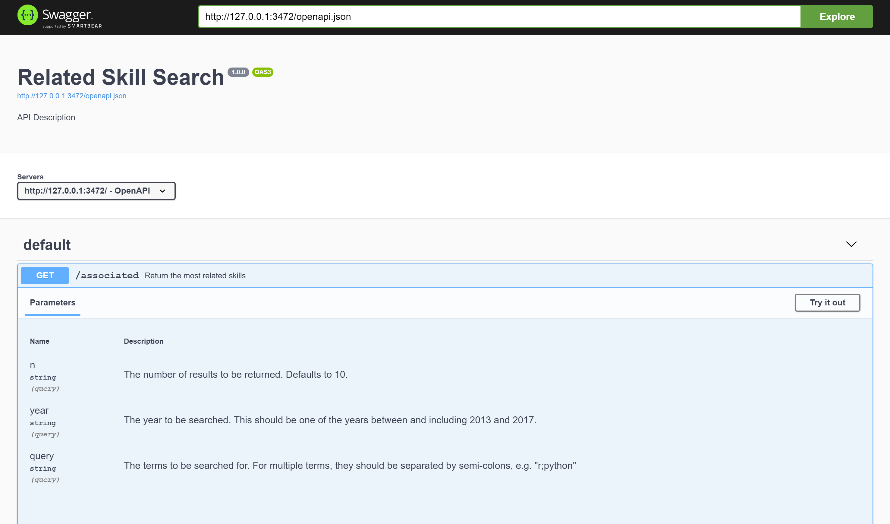
It works!
Putting our API onto the interwebz
Now we just need to run our API on a cloud service. I use DigitalOcean because the analogsea package makes everything such a breeze. Speaking of things being breezy, there’s even a special command, within plumber, to provision a DigitalOcean instance to deploy a plumber API specifically. Here’s how I did that below.
I found that uploading the big database would occasionally fail. So I put it on Dropbox, shared it, and modified the URL slightly (according to some guide I found) to be able to download it with wget. See the code below for how.
droplet <- plumber::do_provision(region="ams3", size="s-1vcpu-3gb",
                            unstable = TRUE, example = FALSE)

Sys.sleep(10) # wait to make sure everything finishes first

analogsea::install_r_package(droplet, package = "dplyr")
analogsea::install_r_package(droplet, package = "tidyr")
analogsea::install_r_package(droplet, package = "purrr")
analogsea::install_r_package(droplet, package = "dbplyr")
analogsea::install_r_package(droplet, package = "DBI")
analogsea::install_r_package(droplet, package = "RSQLite")
analogsea::install_r_package(droplet, package = "stringdist")
analogsea::install_r_package(droplet, package = "stringr")

analogsea::droplet_ssh(droplet, "wget https://www.dropbox.com/s/########/termsdb.sqlite?dl=1")
analogsea::droplet_ssh(droplet, "mv termsdb.sqlite?dl=1 /root/termsdb.sqlite")

plumber::do_deploy_api(droplet = droplet,
              path = "skills",
              localPath = getwd(),
              swagger = TRUE,
              port = 8005)
Aaaaand … drumroll … we have an API on the interwebz! Unfortunately, I never managed to make the Swagger graphical interface accessible online - not quite sure what I missed. But the API worked just fine. I could test it by curling some responses.
library(curl)
library(jsonlite)

# Associated
fromJSON(
  curl("http://165.22.193.221/skills/associated?year=2013&query=r;statistik"))

# Checkterms
fromJSON(
  curl("http://165.22.193.221/skills/checkterm?query=måleri"))

# Random
fromJSON(
  curl("http://165.22.193.221/skills/random"))
Next Steps
So, the next thing to do will be to turn this into a Shiny app. That’s also not something I’ve done before, but I’m really looking forward to giving it a shot. I spoke to the JobTech people, and they had a great suggestion to turn it into a network visualisation too, to give an idea of clusters of skills, which should be another layer of usefulness.
I’ll update here when that’s up and working!
EDIT: Shiny app is up and running here.
Conclusions
So, in summary, here I turned 4.2 million texts into a useful tool, that responds reasonably quickly. The actual method itself is embarrassingly simple, but the difficult part was doing it all at such scale. Using the incredible DBI, dbplyr, RSQLite and plumber packages, the process from turning this from a prototype into a working API, theoretically ready for production, was surprisingly quick and painless.
I’ll update this case study when I’ve had a chance to build this into a fun little shiny app too! Looking forward to digging my teeth into that too!