TOC
Background
A while back, I was messing about with a simple pharmacological model called the Hill function in order to figure out the syntax for nonlinear modelling using several different tools in R. The exercise was helpful for me, and I’ve gone back to it several times to grab the syntax for new applications, so I thought I’d write it up for others (and also so I don’t have to go and find it each time on my own computer..).
#remotes::install_github("mathesong/kinfitr")

library(tidyverse)
## -- Attaching packages ---------------------------------------------------------------------- tidyverse 1.3.0 --## v ggplot2 3.3.0 v purrr 0.3.3
## v tibble 3.0.0 v dplyr 0.8.5
## v tidyr 1.0.2 v stringr 1.4.0
## v readr 1.3.1 v forcats 0.5.0## -- Conflicts ------------------------------------------------------------------------- tidyverse_conflicts() --
## x dplyr::filter() masks stats::filter()
## x dplyr::lag() masks stats::lag()library(kinfitr)
library(nls.multstart)
library(nlme)##
## Attaching package: 'nlme'## The following object is masked from 'package:dplyr':
##
## collapselibrary(brms)## Loading required package: Rcpp## Loading 'brms' package (version 2.12.0). Useful instructions
## can be found by typing help('brms'). A more detailed introduction
## to the package is available through vignette('brms_overview').##
## Attaching package: 'brms'## The following object is masked from 'package:stats':
##
## arlibrary(hrbrthemes)
library(broom)
library(viridis)## Loading required package: viridisLitecolourcodes <- c("#d4a665", "#d27fff", "#7fd9ff")
colourpal <- c(NLS="#d4a665", NLME="#d27fff", MCMC="#7fd9ff")
theme_set(hrbrthemes::theme_ipsum_rc())The Application, the Model and the Data
Application
In my field of PET pharmacokinetic modelling, we need to correct a set of measurements of blood radioactivity for several factors, which are themselves curves which are measured over time (more about that here). It’s worth noting that these measurements can be made with a sometimes substantial degree of error: there can be mistakes made, or failures of the apparatus.
Model
The Hill Function is one of the models we use for modelling the remaining proportion of the tracer which is not metabolised. This is called the parent fraction.
Data
The data I’ll use here comes from a dataset of [\(^{11}\)C]PBR28 data. The data can be found in the kinfitr package using the following:
data(pbr28)And looking in the Metabolite section of each individual’s JSON data. Note that the durations are set to zero, because they were never recorded.
pbr28$jsondata[[1]]$Metabolite## $Data
## $Data$Values
## [,1] [,2] [,3]
## [1,] 0 0 1.0000
## [2,] 60 0 0.9900
## [3,] 180 0 0.9635
## [4,] 300 0 0.8796
## [5,] 630 0 0.4405
## [6,] 1200 0 0.2398
## [7,] 2400 0 0.0954
## [8,] 3600 0 0.0755
## [9,] 5400 0 0.0712
##
## $Data$Type
## [1] "plasmaParentFraction"
##
## $Data$Method
## [1] "HPLC"
##
## $Data$Labels
## [1] "sampleStartTime" "sampleDuration" "parentFraction"
##
## $Data$units
## [1] "s" "s" "fraction"So, now let’s put everything together a little bit more neatly.
extract_metabolite <- function(jsondata) {
  suppressMessages(
    parentFraction <- as_tibble(jsondata$Metabolite$Data$Values,
                                .name_repair = "unique")
  )
  names(parentFraction) = jsondata$Metabolite$Data$Labels
  parentFraction$Time = with(parentFraction,
                             sampleStartTime + 0.5*sampleDuration)
  parentFraction <- select(parentFraction, Time, parentFraction)
  return(parentFraction)
}

pfdata <- pbr28 %>%
  mutate(pf = map(jsondata, extract_metabolite)) %>%
  select(PET, Subjname, PETNo, Genotype, pf)
Fitting using nonlinear least squares (NLS)
First, I’ll go through how to fit these curves one by one using NLS. This is the most common way that this is currently performed in the field. NLS makes use of gradient descent to find the set of parameters which maximise the likelihood of the data under them. We can analogise this by considering the algorithm hopping around parameter space to find the lowest point (i.e. with the lowest ‘cost’ - the residual sum of squares). We could do this by exploring a grid of potential parameter values, but this is extremely inefficient, and would only be as fine-grained as our grid was. Instead, the direction and size of the jumps are determined by the gradients of the cost function below its feet, i.e. if it feels that it’s on a downhill, it will jump in the direction that takes it down fastest. It will stop jumping when it feels that it is flat underfoot, and that all directions go upwards.
So, gradient descent is more efficient than a grid of locations. However, gradient descent can land in so-called local minima. These are positions that are the minimum in their local neighbourhood, but not the lowest point in the whole of parameter space. To get around this problem, and to avoid fitting failures, we can fit the model multiple times, starting in different locations, and choose the one with the best fit: that’s what the nls.multstart package does. This package uses the minpack.lm package under the hood, which makes use of the Levenberg–Marquardt algorithm, and fits with a set of different starting parameters.
Fitting a single curve
First let’s take a look at how the data look
pfdat <- pfdata$pf[[1]]

ggplot(pfdat, aes(x=Time, y=parentFraction)) +
  geom_point(size=3) +
  ylim(c(0, 1))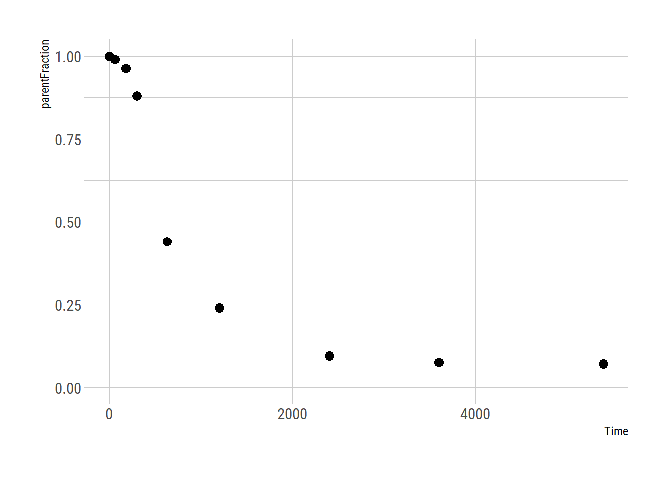
And let’s define the function. Note that kinfitr does contain the Hill function, and additionally contains extra optional parameters for if the decrease begins at a time other than 0, or if curve may not start at 1 (kinfitr::metab_hill()). But we’ll define it ourselves for the purpose of this exercise.
hillfunc <- function(Time, a, b, c) {
  1 - ( ( (1-a) * Time^b) / ( c + (Time)^b ) )
}
… and let’s fit it. I’ll show off two methods. I’ll use the nls.multstart package first, which fits the function with different starting parameters so that we don’t have to worry too much about not defining good enough starting parameters.
hill_nls_fit <- nls.multstart::nls_multstart(parentFraction ~ hillfunc(Time, a, b, c),
                             data = pfdat,
                             lower=c(a=0, b=1, c=0),
                             upper=c(a=1, b=Inf, c=1e12),
                             start_lower = c(a=0, b=1, c=0),
                             start_upper = c(a=0.5, b=500, c=1e12),
                             iter = 500,
                             supp_errors = "Y")
and let’s check the fit
summary(hill_nls_fit)##
## Formula: parentFraction ~ hillfunc(Time, a, b, c)
##
## Parameters:
## Estimate Std. Error t value Pr(>|t|)
## a 7.931e-02 1.762e-02 4.501 0.0041 **
## b 2.619e+00 2.507e-01 10.445 4.52e-05 ***
## c 1.619e+07 2.543e+07 0.637 0.5479
## ---
## Signif. codes: 0 '***' 0.001 '**' 0.01 '*' 0.05 '.' 0.1 ' ' 1
##
## Residual standard error: 0.02753 on 6 degrees of freedom
##
## Number of iterations to convergence: 61
## Achieved convergence tolerance: 1.49e-08plot_nls <- function(nls_object, data) {
predframe <- tibble(Time=seq(from=min(data$Time), to=max(data$Time),
length.out = 1024)) %>%
mutate(ParentFrac = predict(nls_object, newdata = list(Time=.$Time)))
ggplot(data, aes(x=Time, y=parentFraction)) +
geom_point(size=3) +
geom_line(data = predframe, aes(x=Time, y=ParentFrac))
}
plot_nls(hill_nls_fit, pfdat)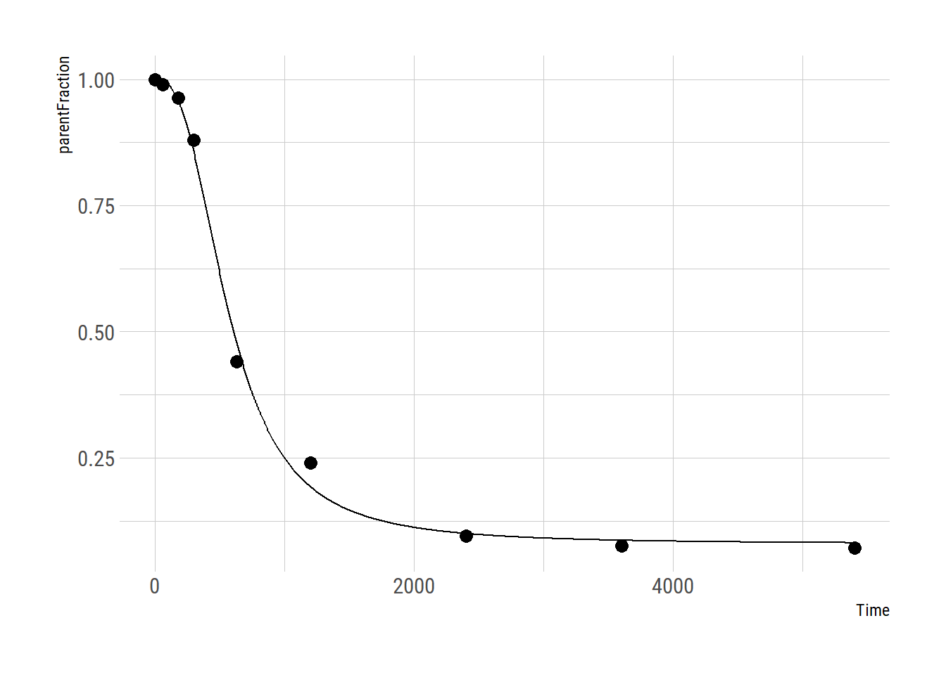
Looks pretty ok! Because the c estimate is so high, we might have some issues with finding it, and with defining a prior for it. I’ll just define it on the log scale instead.
Let’s just run that again then.
hillfunc <- function(Time, a, b, c) {
  1 - ( ( (1-a) * Time^b) / ( 10^c + (Time)^b ) )
}
… and let’s fit it.
hill_nls_fit <- nls.multstart::nls_multstart(parentFraction ~ hillfunc(Time, a, b, c),
                             data = pfdat,
                             lower=c(a=0, b=1, c=0),
                             upper=c(a=1, b=Inf, c=12),
                             start_lower = c(a=0, b=1, c=0),
                             start_upper = c(a=0.5, b=500, c=12),
                             iter = 500,
                             supp_errors = "Y")
and let’s check the fit
summary(hill_nls_fit)##
## Formula: parentFraction ~ hillfunc(Time, a, b, c)
##
## Parameters:
## Estimate Std. Error t value Pr(>|t|)
## a 0.07931 0.01762 4.501 0.0041 **
## b 2.61855 0.25070 10.445 4.52e-05 ***
## c 7.20926 0.68216 10.568 4.22e-05 ***
## ---
## Signif. codes: 0 '***' 0.001 '**' 0.01 '*' 0.05 '.' 0.1 ' ' 1
##
## Residual standard error: 0.02753 on 6 degrees of freedom
##
## Number of iterations to convergence: 75
## Achieved convergence tolerance: 1.49e-08plot_nls(hill_nls_fit, pfdat)
Great - that seems to work fine!
Another way that we could do things would be to use minpack.lm. However, here we have to define our starting parameters more carefully.
If I do as follows, with some thumb-suck starting parameters
hill_nls_fit2 <- minpack.lm::nlsLM(parentFraction ~ hillfunc(Time, a, b, c),
                             data = pfdat,
                             lower=c(a=0, b=1, c=0),
                             upper=c(a=1, b=Inf, c=12),
                             start=c(a=0.5, b=10, c=2))
I get the error
Error in nlsModel(formula, mf, start, wts) :
  singular gradient matrix at initial parameter estimates
This usually either means that our model isn’t working correctly (usually an error in our model definition), or that our starting parameters are too far from reasonable ones. In this case, it’s the latter. So let’s try with some better parameters:
hill_nls_fit2 <- minpack.lm::nlsLM(parentFraction ~ hillfunc(Time, a, b, c),
                             data = pfdat,
                             lower=c(a=0, b=1, c=0),
                             upper=c(a=1, b=Inf, c=12),
                             start=c(a=0.5, b=5, c=5))
That works! And how do the values compare to our multstart values?
coef(hill_nls_fit) # multstart## a b c
## 0.07931366 2.61855033 7.20925556coef(hill_nls_fit2) # not multstart ## a b c
## 0.07931349 2.61854720 7.20924748Basically the same!
Fitting all the cuves
So, now let’s use purrr to fit all the curves.
hill_nls_fit_func <- function(pf_df) {
  nls.multstart::nls_multstart(parentFraction ~ hillfunc(Time, a, b, c),
                             data = pf_df,
                             lower=c(a=0, b=1, c=0),
                             upper=c(a=1, b=Inf, c=12),
                             start_lower = c(a=0, b=1, c=0),
                             start_upper = c(a=0.5, b=500, c=12),
                             iter=500,
                             supp_errors = "Y")
}

pfdata <- pfdata %>%
  mutate(hill_nls_fit = map(pf, ~hill_nls_fit_func(.x)))
Let’s check a couple of fits to make sure things went ok
plot_nls( pfdata$hill_nls_fit[[3]], pfdata$pf[[3]])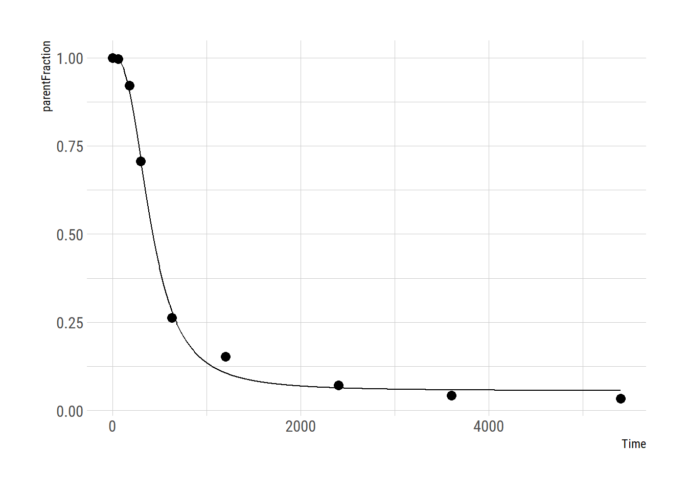
plot_nls( pfdata$hill_nls_fit[[8]], pfdata$pf[[8]])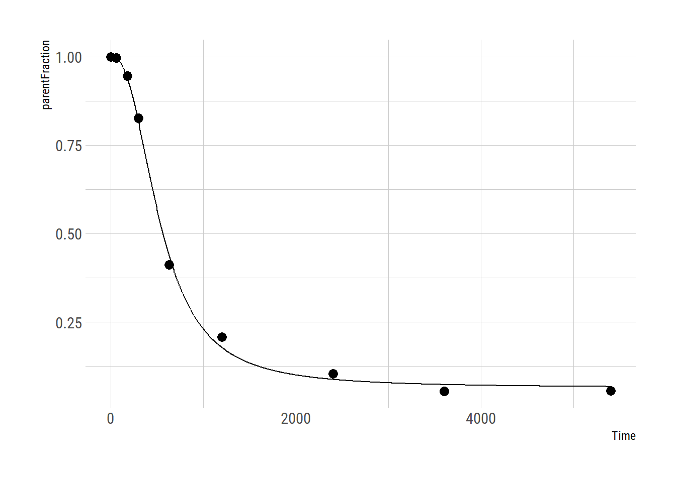
plot_nls( pfdata$hill_nls_fit[[12]], pfdata$pf[[12]])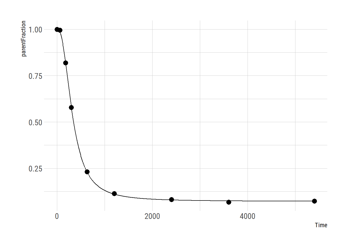
And let’s check the distribution of the outcomes.
hill_nls_outcomes <- pfdata %>%
  mutate(outpars = map(hill_nls_fit, ~broom::tidy(.x))) %>%
  select(-pf, -hill_nls_fit) %>%
  unnest(cols="outpars")

ggplot(hill_nls_outcomes, aes(x=estimate, colour=term, fill=term)) +
  geom_density(alpha=0.5, fill=colourcodes[1], colour=colourcodes[1]) +
  facet_wrap(~term, scales = "free")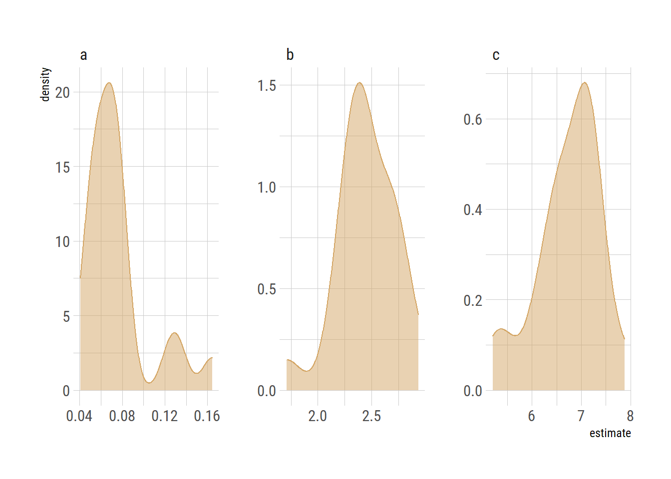
hill_nls_outcomes_summary <- hill_nls_outcomes %>%
  group_by(term) %>%
  summarise(mean = mean(estimate),
            median = median(estimate),
            sd = sd(estimate)) %>%
  ungroup()

knitr::kable(hill_nls_outcomes_summary, digits = 3)| term | mean | median | sd |
|---|---|---|---|
| a | 0.076 | 0.069 | 0.031 |
| b | 2.452 | 2.434 | 0.272 |
| c | 6.739 | 6.929 | 0.657 |
Fits
And we can check the fits
hill_nls_plots <- pfdata %>%
  select(PET, pf) %>%
  unnest(pf)

hill_predtimes <- tidyr::crossing(PET=pfdata$PET,
                              Time=seq(min(hill_nls_plots$Time),
                                  max(hill_nls_plots$Time),
                                  length.out=128))

hill_nlspreds <- hill_predtimes %>%
  group_by(PET) %>%
  nest(preds = Time) %>%
  left_join(select(pfdata, PET, hill_nls_fit)) %>%
  mutate(preds = map2(preds, hill_nls_fit, ~broom::augment(.y, newdata=.x))) %>%
  select(-hill_nls_fit) %>%
  ungroup() %>%
  unnest(cols=preds)
## Joining, by = "PET"ggplot(hill_nls_plots, aes(x=Time, y=parentFraction)) +
geom_point() +
geom_line(data=hill_nlspreds, aes(y=.fitted), colour=colourcodes[1], size=0.7) +
facet_wrap(~PET, ncol=4) +
theme(axis.text.x = element_text(angle = 45, hjust = 1))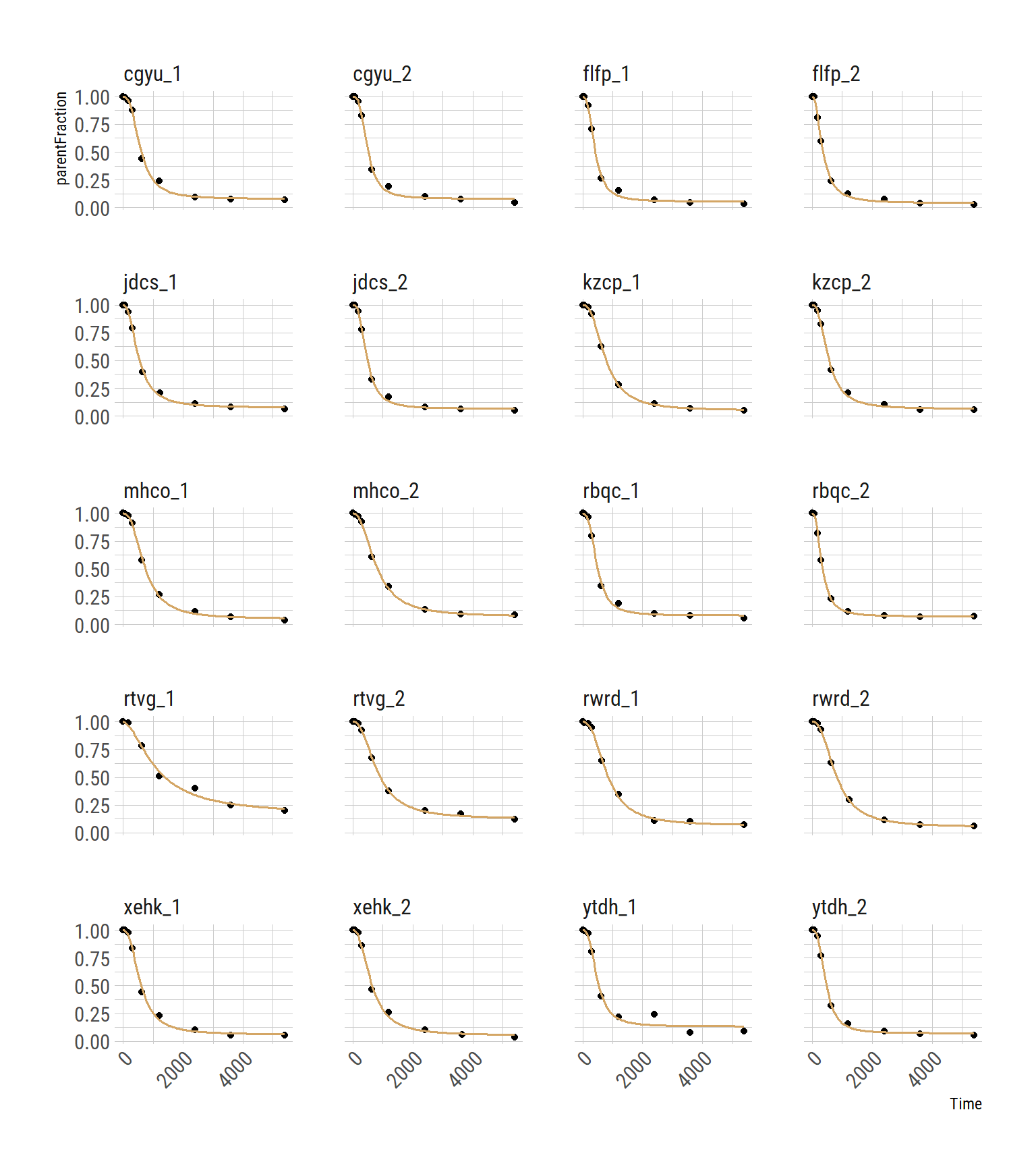
NLS Summary
What we have done is to fit each curve, separately. The fits look pretty good. It’s worth noting that the second-to-last measurement, ytdh_1, has a pretty bad data point around the middle. This pulls the fitted curve towards it, and it overshoots the last two points. This is quite annoying, and not to easy to fix. We could choose to remove the point. Or just leave it and accept some degree of error.
Doing our modelling in this way, so-called fixed effects regression, is, in the words of Richard McElreath, equivalent to giving our model anterograde amnesia. The curves are all fairly similar, however instead of learning anything about what reasonable values of the parameters are following fitting of each curve, we instead completely wipe the memory of our model before it fits each new curve. So, this is why we would hope that a multilevel approach might do a better job.
Fitting using frequentist multilevel modelling (nlme)
Here, we use a multilevel modelling approach, but still using maximum likelihood. I’ll use the nlme package here. While this functionality does exist in lme4, the nonlinear syntax was always a bit unintuitive for me. What we are doing is telling the model that each of the parameters is sampled from a normal distribution across individuals. In this way, the model can pull unlikely parameter values back towards the mean of the distribution. In addition, the correlations between the parameters are estimated, which allows the model to learn about likely values of each parameter based on the values of the other parameters, and constrain the selection of unlikely values in this way too.
Just a note: for simplicity’s sake, I will model all measurements as being derived from a common normal distribution, i.e. nested within measurements. However, of the 20 measurements, these come from 10 individuals, with 2 measurements within each individual. We could have fit this instead, but this is less common, and the point of this exercise is to go through the syntax.
Fitting the model to everyone
So, now we fit everything at once. Let’s first prepare the data in a long, unnested form.
pf_modeldata <- pfdata %>%
  select(PET:pf) %>%
  unnest(cols="pf")

head(pf_modeldata, n = 12)
## # A tibble: 12 x 6
## PET Subjname PETNo Genotype Time parentFraction
## <chr> <chr> <dbl> <chr> <dbl> <dbl>
## 1 cgyu_1 cgyu 1 MAB 0 1
## 2 cgyu_1 cgyu 1 MAB 60 0.99
## 3 cgyu_1 cgyu 1 MAB 180 0.964
## 4 cgyu_1 cgyu 1 MAB 300 0.880
## 5 cgyu_1 cgyu 1 MAB 630 0.440
## 6 cgyu_1 cgyu 1 MAB 1200 0.240
## 7 cgyu_1 cgyu 1 MAB 2400 0.0954
## 8 cgyu_1 cgyu 1 MAB 3600 0.0755
## 9 cgyu_1 cgyu 1 MAB 5400 0.0712
## 10 cgyu_2 cgyu 2 MAB 0 1
## 11 cgyu_2 cgyu 2 MAB 60 0.996
## 12 cgyu_2 cgyu 2 MAB 180 0.958Now let’s fit the model!
hill_nlme_fit <- nlme(parentFraction ~ hillfunc(Time, a, b, c),
                  data = pf_modeldata,
                  fixed=a + b + c ~ 1,
                  random = a + b + c ~ 1,
                  groups = ~ PET,
                  start = hill_nls_outcomes_summary$mean,
                  verbose = F)

summary(hill_nlme_fit)
## Nonlinear mixed-effects model fit by maximum likelihood
## Model: parentFraction ~ hillfunc(Time, a, b, c)
## Data: pf_modeldata
## AIC BIC logLik
## -686.7261 -654.9083 353.3631
##
## Random effects:
## Formula: list(a ~ 1, b ~ 1, c ~ 1)
## Level: PET
## Structure: General positive-definite, Log-Cholesky parametrization
## StdDev Corr
## a 0.01725372 a b
## b 0.25329033 -0.620
## c 0.58963922 -0.554 0.900
## Residual 0.02341274
##
## Fixed effects: a + b + c ~ 1
## Value Std.Error DF t-value p-value
## a 0.072428 0.00536268 156 13.50602 0
## b 2.404842 0.07159599 156 33.58906 0
## c 6.611691 0.17656779 156 37.44562 0
## Correlation:
## a b
## b -0.138
## c -0.076 0.936
##
## Standardized Within-Group Residuals:
## Min Q1 Med Q3 Max
## -2.44880864 -0.35347381 0.01844329 0.45900088 5.18383085
##
## Number of Observations: 178
## Number of Groups: 20And let’s check out the parameters
nlme_coef = as_tibble(coef(hill_nlme_fit), rownames = 'PET')
nlme_coef
## # A tibble: 20 x 4
## PET a b c
## <chr> <dbl> <dbl> <dbl>
## 1 cgyu_1 0.0717 2.48 6.85
## 2 cgyu_2 0.0678 2.64 7.10
## 3 flfp_1 0.0579 2.64 6.89
## 4 flfp_2 0.0595 2.42 6.14
## 5 jdcs_1 0.0765 2.34 6.33
## 6 jdcs_2 0.0638 2.60 6.94
## 7 kzcp_1 0.0617 2.46 7.06
## 8 kzcp_2 0.0678 2.46 6.69
## 9 mhco_1 0.0621 2.46 6.99
## 10 mhco_2 0.0757 2.28 6.57
## 11 rbqc_1 0.0702 2.58 6.91
## 12 rbqc_2 0.0713 2.46 6.18
## 13 rtvg_1 0.116 1.61 4.99
## 14 rtvg_2 0.0970 2.09 6.12
## 15 rwrd_1 0.0694 2.38 6.92
## 16 rwrd_2 0.0646 2.41 6.95
## 17 xehk_1 0.0667 2.44 6.71
## 18 xehk_2 0.0659 2.40 6.66
## 19 ytdh_1 0.0983 2.32 6.27
## 20 ytdh_2 0.0652 2.62 6.97Fits
And we can check the fits
hill_nlmepreds <- hill_predtimes %>%
  mutate(.fitted=predict(hill_nlme_fit, newdata=hill_predtimes))

ggplot(pf_modeldata, aes(x=Time, y=parentFraction)) +
  geom_point() +
  geom_line(data=hill_nlmepreds, aes(y=.fitted), colour=colourcodes[2], size=0.7) +
  facet_wrap(~PET, ncol=4)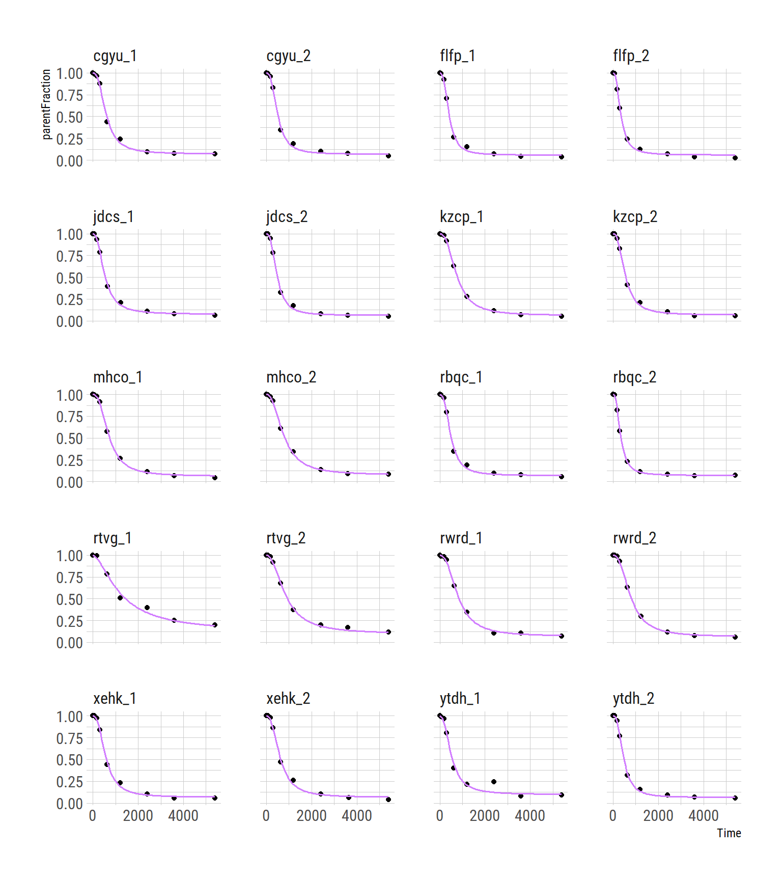
And we can compare them to the NLS outcomes
nlme_coef_tidy <- nlme_coef %>%
  gather(Parameter, Estimate, -PET) %>%
  mutate(Model = "NLME")

nls_coef_tidy <- hill_nls_outcomes %>%
  select(PET, Parameter=term, Estimate=estimate) %>%
  mutate(Model = "NLS")

nls_nlme_comparison <- full_join(nls_coef_tidy, nlme_coef_tidy)
## Joining, by = c("PET", "Parameter", "Estimate", "Model")ggplot(nls_nlme_comparison, aes(x=Estimate, colour=Model, fill=Model)) +
geom_density(alpha=0.3) +
scale_colour_manual(values=colourpal) +
scale_fill_manual(values=colourpal) +
facet_wrap(~Parameter, scales="free")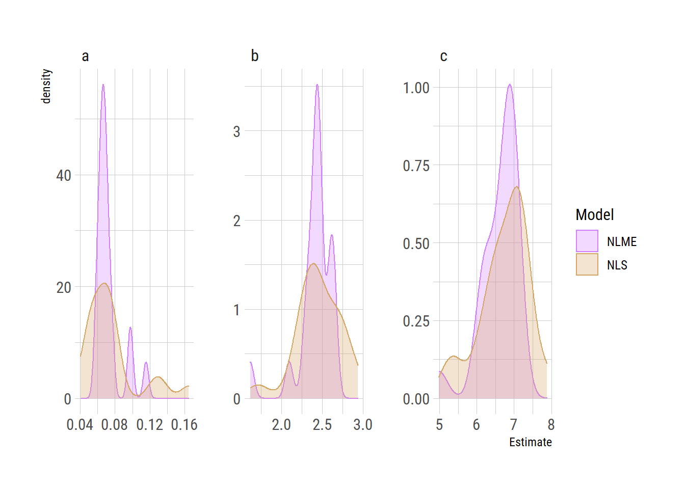
We can see that the NLME density is much peakier, showing the shrinkage: values are being pulled towards the centre based on the lessons learned by fitting the whole sample together.
NLME Summary
We can see the effect of the shrinkage immediately in the second-to-last curve, which was problematic before, as well as in the distributions of the parameters. So that’s nice! But now let’s go deeper.
Bayesian multilevel modelling using MCMC with brms
So, now we are going to model the same curves, but using Markov Chain Monte Carlo (MCMC) instead of maximum likelihood. This requires that we set priors on our parameters (which gives us the opportunity to include all the things we know about our parameters a priori). Then the algorithm traverses parameter space, spending time in any particular region in proportion to its relative posterior probability. This allows us to build up a posterior probability distribution over each parameter, and to make inferences using the probabilities themselves.
We use MCMC with STAN under the hood, and brms gives us a convenient interface, which writes all the STAN code for us and makes our lives easier - at least when the model is simple enough to be written using brms syntax.
Because the purpose of this exercise here is mostly to grok the syntax, I’ve just used priors which are based on the same dataset. This is not what you should be doing in practice.
Modelling a single curve
Let’s first just try a single curve for simplicity’s sake.
hillprior <- c(
  set_prior("normal(0.2, 0.1)", nlpar = "a", lb=0, ub=1),
  set_prior("normal(2, 1)", nlpar = "b", lb=1),
  set_prior("normal(7, 3)", nlpar = "c", lb=0),
  set_prior("normal(0.05, 0.2)", class="sigma"))

hill_bayes_fit_formula <- bf(parentFraction ~ 1 - ( ( (1-a) * Time^b) /
                                                      ( 10^c + (Time)^b ) ),
     # Nonlinear variables
     a + b + c ~ 1,
     # Nonlinear fit
     nl = TRUE)

hill_bayes_fit <- brm(
  hill_bayes_fit_formula,
  family=gaussian(),
  data = pfdat,
  prior = hillprior )
## Compiling the C++ model## Start sampling##
## SAMPLING FOR MODEL '22df16fab4ad9b8db3198565904815ba' NOW (CHAIN 1).
## Chain 1:
## Chain 1: Gradient evaluation took 0 seconds
## Chain 1: 1000 transitions using 10 leapfrog steps per transition would take 0 seconds.
## Chain 1: Adjust your expectations accordingly!
## Chain 1:
## Chain 1:
## Chain 1: Iteration: 1 / 2000 [ 0%] (Warmup)
## Chain 1: Iteration: 200 / 2000 [ 10%] (Warmup)
## Chain 1: Iteration: 400 / 2000 [ 20%] (Warmup)
## Chain 1: Iteration: 600 / 2000 [ 30%] (Warmup)
## Chain 1: Iteration: 800 / 2000 [ 40%] (Warmup)
## Chain 1: Iteration: 1000 / 2000 [ 50%] (Warmup)
## Chain 1: Iteration: 1001 / 2000 [ 50%] (Sampling)
## Chain 1: Iteration: 1200 / 2000 [ 60%] (Sampling)
## Chain 1: Iteration: 1400 / 2000 [ 70%] (Sampling)
## Chain 1: Iteration: 1600 / 2000 [ 80%] (Sampling)
## Chain 1: Iteration: 1800 / 2000 [ 90%] (Sampling)
## Chain 1: Iteration: 2000 / 2000 [100%] (Sampling)
## Chain 1:
## Chain 1: Elapsed Time: 1.159 seconds (Warm-up)
## Chain 1: 1.717 seconds (Sampling)
## Chain 1: 2.876 seconds (Total)
## Chain 1:
##
## SAMPLING FOR MODEL '22df16fab4ad9b8db3198565904815ba' NOW (CHAIN 2).
## Chain 2:
## Chain 2: Gradient evaluation took 0 seconds
## Chain 2: 1000 transitions using 10 leapfrog steps per transition would take 0 seconds.
## Chain 2: Adjust your expectations accordingly!
## Chain 2:
## Chain 2:
## Chain 2: Iteration: 1 / 2000 [ 0%] (Warmup)
## Chain 2: Iteration: 200 / 2000 [ 10%] (Warmup)
## Chain 2: Iteration: 400 / 2000 [ 20%] (Warmup)
## Chain 2: Iteration: 600 / 2000 [ 30%] (Warmup)
## Chain 2: Iteration: 800 / 2000 [ 40%] (Warmup)
## Chain 2: Iteration: 1000 / 2000 [ 50%] (Warmup)
## Chain 2: Iteration: 1001 / 2000 [ 50%] (Sampling)
## Chain 2: Iteration: 1200 / 2000 [ 60%] (Sampling)
## Chain 2: Iteration: 1400 / 2000 [ 70%] (Sampling)
## Chain 2: Iteration: 1600 / 2000 [ 80%] (Sampling)
## Chain 2: Iteration: 1800 / 2000 [ 90%] (Sampling)
## Chain 2: Iteration: 2000 / 2000 [100%] (Sampling)
## Chain 2:
## Chain 2: Elapsed Time: 0.84 seconds (Warm-up)
## Chain 2: 0.881 seconds (Sampling)
## Chain 2: 1.721 seconds (Total)
## Chain 2:
##
## SAMPLING FOR MODEL '22df16fab4ad9b8db3198565904815ba' NOW (CHAIN 3).
## Chain 3:
## Chain 3: Gradient evaluation took 0 seconds
## Chain 3: 1000 transitions using 10 leapfrog steps per transition would take 0 seconds.
## Chain 3: Adjust your expectations accordingly!
## Chain 3:
## Chain 3:
## Chain 3: Iteration: 1 / 2000 [ 0%] (Warmup)
## Chain 3: Iteration: 200 / 2000 [ 10%] (Warmup)
## Chain 3: Iteration: 400 / 2000 [ 20%] (Warmup)
## Chain 3: Iteration: 600 / 2000 [ 30%] (Warmup)
## Chain 3: Iteration: 800 / 2000 [ 40%] (Warmup)
## Chain 3: Iteration: 1000 / 2000 [ 50%] (Warmup)
## Chain 3: Iteration: 1001 / 2000 [ 50%] (Sampling)
## Chain 3: Iteration: 1200 / 2000 [ 60%] (Sampling)
## Chain 3: Iteration: 1400 / 2000 [ 70%] (Sampling)
## Chain 3: Iteration: 1600 / 2000 [ 80%] (Sampling)
## Chain 3: Iteration: 1800 / 2000 [ 90%] (Sampling)
## Chain 3: Iteration: 2000 / 2000 [100%] (Sampling)
## Chain 3:
## Chain 3: Elapsed Time: 1.003 seconds (Warm-up)
## Chain 3: 0.36 seconds (Sampling)
## Chain 3: 1.363 seconds (Total)
## Chain 3:
##
## SAMPLING FOR MODEL '22df16fab4ad9b8db3198565904815ba' NOW (CHAIN 4).
## Chain 4:
## Chain 4: Gradient evaluation took 0 seconds
## Chain 4: 1000 transitions using 10 leapfrog steps per transition would take 0 seconds.
## Chain 4: Adjust your expectations accordingly!
## Chain 4:
## Chain 4:
## Chain 4: Iteration: 1 / 2000 [ 0%] (Warmup)
## Chain 4: Iteration: 200 / 2000 [ 10%] (Warmup)
## Chain 4: Iteration: 400 / 2000 [ 20%] (Warmup)
## Chain 4: Iteration: 600 / 2000 [ 30%] (Warmup)
## Chain 4: Iteration: 800 / 2000 [ 40%] (Warmup)
## Chain 4: Iteration: 1000 / 2000 [ 50%] (Warmup)
## Chain 4: Iteration: 1001 / 2000 [ 50%] (Sampling)
## Chain 4: Iteration: 1200 / 2000 [ 60%] (Sampling)
## Chain 4: Iteration: 1400 / 2000 [ 70%] (Sampling)
## Chain 4: Iteration: 1600 / 2000 [ 80%] (Sampling)
## Chain 4: Iteration: 1800 / 2000 [ 90%] (Sampling)
## Chain 4: Iteration: 2000 / 2000 [100%] (Sampling)
## Chain 4:
## Chain 4: Elapsed Time: 0.846 seconds (Warm-up)
## Chain 4: 1.131 seconds (Sampling)
## Chain 4: 1.977 seconds (Total)
## Chain 4:## Warning: There were 83 divergent transitions after warmup. Increasing adapt_delta above 0.8 may help. See
## http://mc-stan.org/misc/warnings.html#divergent-transitions-after-warmup## Warning: Examine the pairs() plot to diagnose sampling problems## Warning: Bulk Effective Samples Size (ESS) is too low, indicating posterior means and medians may be unreliable.
## Running the chains for more iterations may help. See
## http://mc-stan.org/misc/warnings.html#bulk-essWe have some divergent transitions. This would usually be something to look into, but this guide is about the syntax, so we’ll ignore that for today.
Let’s check the fit!
summary(hill_bayes_fit)## Warning: There were 83 divergent transitions after warmup. Increasing
## adapt_delta above 0.8 may help. See http://mc-stan.org/misc/
## warnings.html#divergent-transitions-after-warmup## Family: gaussian
## Links: mu = identity; sigma = identity
## Formula: parentFraction ~ 1 - (((1 - a) * Time^b)/(10^c + (Time)^b))
## a ~ 1
## b ~ 1
## c ~ 1
## Data: pfdat (Number of observations: 9)
## Samples: 4 chains, each with iter = 2000; warmup = 1000; thin = 1;
## total post-warmup samples = 4000
##
## Population-Level Effects:
## Estimate Est.Error l-95% CI u-95% CI Rhat Bulk_ESS Tail_ESS
## a_Intercept 0.08 0.02 0.04 0.13 1.01 1067 1021
## b_Intercept 2.70 0.31 2.14 3.35 1.01 585 1306
## c_Intercept 7.42 0.83 5.92 9.18 1.01 580 1272
##
## Family Specific Parameters:
## Estimate Est.Error l-95% CI u-95% CI Rhat Bulk_ESS Tail_ESS
## sigma 0.03 0.01 0.02 0.07 1.01 322 1262
##
## Samples were drawn using sampling(NUTS). For each parameter, Bulk_ESS
## and Tail_ESS are effective sample size measures, and Rhat is the potential
## scale reduction factor on split chains (at convergence, Rhat = 1).plot(hill_bayes_fit)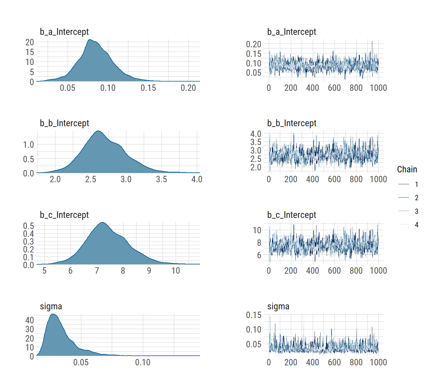
pairs(hill_bayes_fit)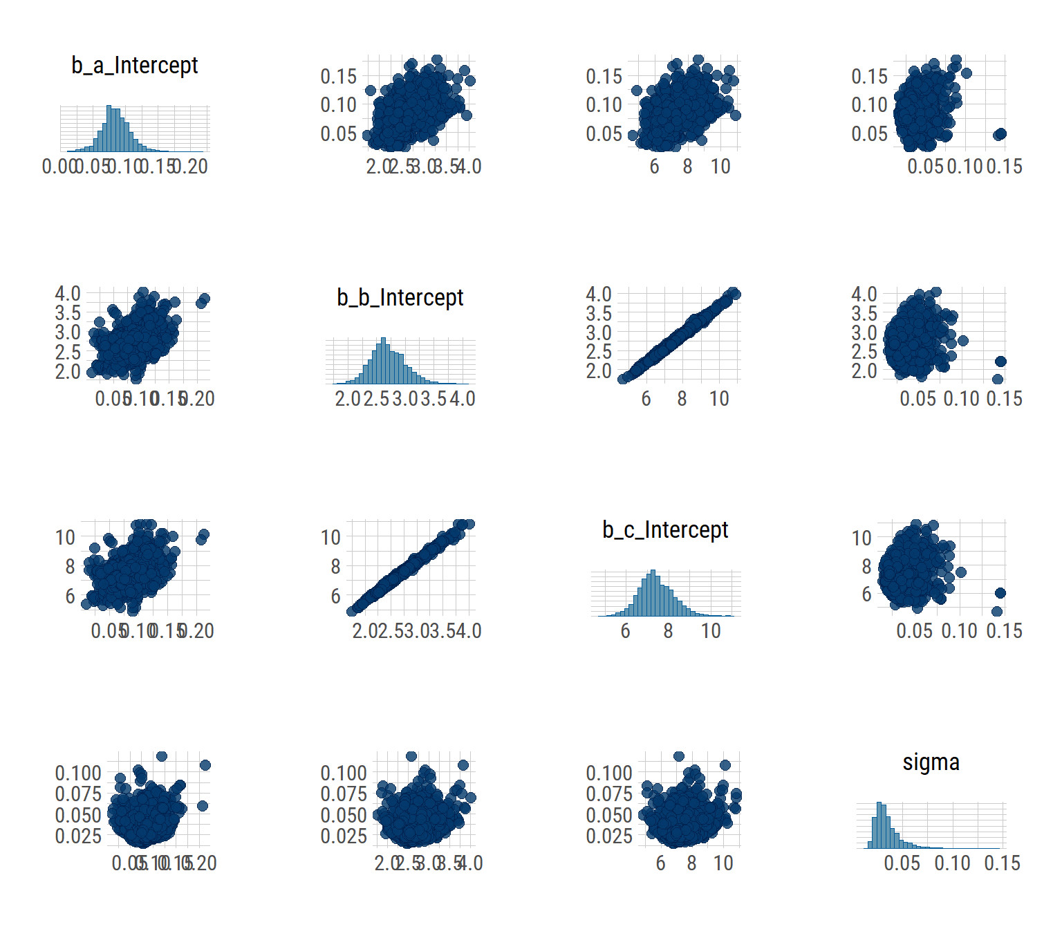
Seems to have done a pretty ok job! We can see that there’s a high degree of correlation between b and c.
predtimes <- unique(hill_predtimes$Time)

hill_bayes_fitted <- fitted(hill_bayes_fit,
                            newdata=list(Time = predtimes)) %>%
  as_tibble()

hill_bayes_pred <- predict(hill_bayes_fit,
                           newdata=list(Time = predtimes)) %>%
  as_tibble()
hill_bayes_ribbons <- tibble(
Time = predtimes,
parentFraction=hill_bayes_fitted$Estimate,
Estimate = hill_bayes_fitted$Estimate,
pred_lower = hill_bayes_pred$Q2.5,
pred_upper = hill_bayes_pred$Q97.5,
fitted_lower = hill_bayes_fitted$Q2.5,
fitted_upper = hill_bayes_fitted$Q97.5)
ggplot(pfdat, aes(x=Time, y=parentFraction)) +
geom_point(size=3) +
geom_ribbon(data=hill_bayes_ribbons, aes(ymin=pred_lower, ymax=pred_upper),
alpha=0.2, fill=colourcodes[3]) +
geom_ribbon(data=hill_bayes_ribbons, aes(ymin=fitted_lower, ymax=fitted_upper),
alpha=0.5, fill=colourcodes[3]) +
geom_line(data=hill_bayes_ribbons, aes(y=Estimate), colour=colourcodes[3],
size=1)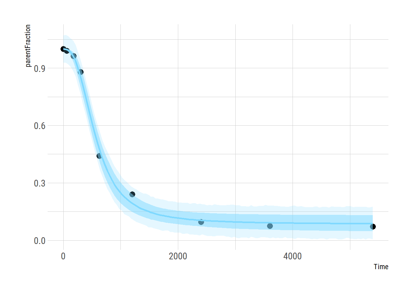
And the fit looks ok too. Here we see the fit, the 95% credible interval (the uncertainty our model has about the line of best fit), and the 95% prediction interval (the interval for our model believes that new data points will fall within with a 95% probability).
Let’s also compare the outcomes between the NLS and the MCMC fit
summary(hill_nls_fit)##
## Formula: parentFraction ~ hillfunc(Time, a, b, c)
##
## Parameters:
## Estimate Std. Error t value Pr(>|t|)
## a 0.07931 0.01762 4.501 0.0041 **
## b 2.61855 0.25070 10.445 4.52e-05 ***
## c 7.20926 0.68216 10.568 4.22e-05 ***
## ---
## Signif. codes: 0 '***' 0.001 '**' 0.01 '*' 0.05 '.' 0.1 ' ' 1
##
## Residual standard error: 0.02753 on 6 degrees of freedom
##
## Number of iterations to convergence: 75
## Achieved convergence tolerance: 1.49e-08summary(hill_bayes_fit)## Warning: There were 83 divergent transitions after warmup. Increasing
## adapt_delta above 0.8 may help. See http://mc-stan.org/misc/
## warnings.html#divergent-transitions-after-warmup## Family: gaussian
## Links: mu = identity; sigma = identity
## Formula: parentFraction ~ 1 - (((1 - a) * Time^b)/(10^c + (Time)^b))
## a ~ 1
## b ~ 1
## c ~ 1
## Data: pfdat (Number of observations: 9)
## Samples: 4 chains, each with iter = 2000; warmup = 1000; thin = 1;
## total post-warmup samples = 4000
##
## Population-Level Effects:
## Estimate Est.Error l-95% CI u-95% CI Rhat Bulk_ESS Tail_ESS
## a_Intercept 0.08 0.02 0.04 0.13 1.01 1067 1021
## b_Intercept 2.70 0.31 2.14 3.35 1.01 585 1306
## c_Intercept 7.42 0.83 5.92 9.18 1.01 580 1272
##
## Family Specific Parameters:
## Estimate Est.Error l-95% CI u-95% CI Rhat Bulk_ESS Tail_ESS
## sigma 0.03 0.01 0.02 0.07 1.01 322 1262
##
## Samples were drawn using sampling(NUTS). For each parameter, Bulk_ESS
## and Tail_ESS are effective sample size measures, and Rhat is the potential
## scale reduction factor on split chains (at convergence, Rhat = 1).Modelling all the curves
Here, I’ll also define the function as a STAN function, just to demonstrate the syntax. Don’t forget those semicolons!
hillstan <- "
  real hill_stan(real Time, real a, real b, real c) {

    real pred;

    pred = 1 - ( ( (1-a) * Time^b) / ( 10^c + (Time)^b ) );

    return(pred);
  }
"

get_prior(bf(parentFraction ~ hill_stan(Time, a, b, c),
     # Nonlinear variables
     a + b + c ~ 1 + (1|k|PET),
     # Nonlinear fit
     nl = TRUE), data=pf_modeldata)
## prior class coef group resp dpar nlpar bound
## 1 lkj(1) cor
## 2 cor PET
## 3 student_t(3, 0, 10) sigma
## 4 b a
## 5 b Intercept a
## 6 student_t(3, 0, 10) sd a
## 7 sd PET a
## 8 sd Intercept PET a
## 9 b b
## 10 b Intercept b
## 11 student_t(3, 0, 10) sd b
## 12 sd PET b
## 13 sd Intercept PET b
## 14 b c
## 15 b Intercept c
## 16 student_t(3, 0, 10) sd c
## 17 sd PET c
## 18 sd Intercept PET chillprior_multilevel <- c(
set_prior("normal(0.2, 0.1)", nlpar = "a", lb=0, ub=1),
set_prior("normal(2, 1)", nlpar = "b", lb=1),
set_prior("normal(7, 3)", nlpar = "c", lb=0),
set_prior("normal(0.05, 0.02)", class="sigma"),
set_prior("normal(0.03, 0.02)", class="sd", nlpar="a"),
set_prior("normal(0.3, 0.1)", class="sd", nlpar="b"),
set_prior("normal(0.7, 0.2)", class="sd", nlpar="c"),
set_prior("lkj(2)", class = "cor"))
hill_multilevelbayes_formula <- bf(parentFraction ~ hill_stan(Time, a, b, c),
# Nonlinear variables
a + b + c ~ 1 + (1|k|PET),
# Nonlinear fit
nl = TRUE)Let’s check the STAN code before fitting it
make_stancode(hill_multilevelbayes_formula,
  family=gaussian(),
  data = pf_modeldata,
  prior = hillprior_multilevel,
  stanvars = stanvar(scode = hillstan,
                     block="functions"))
## // generated with brms 2.12.0
## functions {
##
## real hill_stan(real Time, real a, real b, real c) {
##
## real pred;
##
## pred = 1 - ( ( (1-a) * Time^b) / ( 10^c + (Time)^b ) );
##
## return(pred);
## }
##
## }
## data {
## int<lower=1> N; // number of observations
## vector[N] Y; // response variable
## int<lower=1> K_a; // number of population-level effects
## matrix[N, K_a] X_a; // population-level design matrix
## int<lower=1> K_b; // number of population-level effects
## matrix[N, K_b] X_b; // population-level design matrix
## int<lower=1> K_c; // number of population-level effects
## matrix[N, K_c] X_c; // population-level design matrix
## // covariate vectors for non-linear functions
## vector[N] C_1;
## // data for group-level effects of ID 1
## int<lower=1> N_1; // number of grouping levels
## int<lower=1> M_1; // number of coefficients per level
## int<lower=1> J_1[N]; // grouping indicator per observation
## // group-level predictor values
## vector[N] Z_1_a_1;
## vector[N] Z_1_b_2;
## vector[N] Z_1_c_3;
## int<lower=1> NC_1; // number of group-level correlations
## int prior_only; // should the likelihood be ignored?
## }
## transformed data {
## }
## parameters {
## vector<lower=0,upper=1>[K_a] b_a; // population-level effects
## vector<lower=1>[K_b] b_b; // population-level effects
## vector<lower=0>[K_c] b_c; // population-level effects
## real<lower=0> sigma; // residual SD
## vector<lower=0>[M_1] sd_1; // group-level standard deviations
## matrix[M_1, N_1] z_1; // standardized group-level effects
## cholesky_factor_corr[M_1] L_1; // cholesky factor of correlation matrix
## }
## transformed parameters {
## matrix[N_1, M_1] r_1; // actual group-level effects
## // using vectors speeds up indexing in loops
## vector[N_1] r_1_a_1;
## vector[N_1] r_1_b_2;
## vector[N_1] r_1_c_3;
## // compute actual group-level effects
## r_1 = (diag_pre_multiply(sd_1, L_1) * z_1)';
## r_1_a_1 = r_1[, 1];
## r_1_b_2 = r_1[, 2];
## r_1_c_3 = r_1[, 3];
## }
## model {
## // initialize linear predictor term
## vector[N] nlp_a = X_a * b_a;
## // initialize linear predictor term
## vector[N] nlp_b = X_b * b_b;
## // initialize linear predictor term
## vector[N] nlp_c = X_c * b_c;
## // initialize non-linear predictor term
## vector[N] mu;
## for (n in 1:N) {
## // add more terms to the linear predictor
## nlp_a[n] += r_1_a_1[J_1[n]] * Z_1_a_1[n];
## }
## for (n in 1:N) {
## // add more terms to the linear predictor
## nlp_b[n] += r_1_b_2[J_1[n]] * Z_1_b_2[n];
## }
## for (n in 1:N) {
## // add more terms to the linear predictor
## nlp_c[n] += r_1_c_3[J_1[n]] * Z_1_c_3[n];
## }
## for (n in 1:N) {
## // compute non-linear predictor values
## mu[n] = hill_stan(C_1[n] , nlp_a[n] , nlp_b[n] , nlp_c[n]);
## }
## // priors including all constants
## target += normal_lpdf(b_a | 0.2, 0.1)
## - 1 * log_diff_exp(normal_lcdf(1 | 0.2, 0.1), normal_lcdf(0 | 0.2, 0.1));
## target += normal_lpdf(b_b | 2, 1)
## - 1 * normal_lccdf(1 | 2, 1);
## target += normal_lpdf(b_c | 7, 3)
## - 1 * normal_lccdf(0 | 7, 3);
## target += normal_lpdf(sigma | 0.05, 0.02)
## - 1 * normal_lccdf(0 | 0.05, 0.02);
## target += normal_lpdf(sd_1[1] | 0.03, 0.02)
## - 1 * normal_lccdf(0 | 0.03, 0.02);
## target += normal_lpdf(sd_1[2] | 0.3, 0.1)
## - 1 * normal_lccdf(0 | 0.3, 0.1);
## target += normal_lpdf(sd_1[3] | 0.7, 0.2)
## - 1 * normal_lccdf(0 | 0.7, 0.2);
## target += normal_lpdf(to_vector(z_1) | 0, 1);
## target += lkj_corr_cholesky_lpdf(L_1 | 2);
## // likelihood including all constants
## if (!prior_only) {
## target += normal_lpdf(Y | mu, sigma);
## }
## }
## generated quantities {
## // compute group-level correlations
## corr_matrix[M_1] Cor_1 = multiply_lower_tri_self_transpose(L_1);
## vector<lower=-1,upper=1>[NC_1] cor_1;
## // extract upper diagonal of correlation matrix
## for (k in 1:M_1) {
## for (j in 1:(k - 1)) {
## cor_1[choose(k - 1, 2) + j] = Cor_1[j, k];
## }
## }
## }Looks good! Happy not to have to write this all ourselves! Now let’s fit it.
hill_multilevelbayes_fit <- brm(
  hill_multilevelbayes_formula,
  family=gaussian(),
  data = pf_modeldata,
  prior = hillprior_multilevel,
  stanvars = stanvar(scode = hillstan,
                     block="functions"),
  cores = 4)
## Compiling the C++ model## Start sampling## Warning: There were 7 divergent transitions after warmup. Increasing adapt_delta above 0.8 may help. See
## http://mc-stan.org/misc/warnings.html#divergent-transitions-after-warmup## Warning: There were 1 transitions after warmup that exceeded the maximum treedepth. Increase max_treedepth above 10. See
## http://mc-stan.org/misc/warnings.html#maximum-treedepth-exceeded## Warning: Examine the pairs() plot to diagnose sampling problemsAnd check it.
summary(hill_multilevelbayes_fit)## Warning: There were 7 divergent transitions after warmup. Increasing adapt_delta
## above 0.8 may help. See http://mc-stan.org/misc/warnings.html#divergent-
## transitions-after-warmup## Family: gaussian
## Links: mu = identity; sigma = identity
## Formula: parentFraction ~ hill_stan(Time, a, b, c)
## a ~ 1 + (1 | k | PET)
## b ~ 1 + (1 | k | PET)
## c ~ 1 + (1 | k | PET)
## Data: pf_modeldata (Number of observations: 178)
## Samples: 4 chains, each with iter = 2000; warmup = 1000; thin = 1;
## total post-warmup samples = 4000
##
## Group-Level Effects:
## ~PET (Number of levels: 20)
## Estimate Est.Error l-95% CI u-95% CI Rhat Bulk_ESS
## sd(a_Intercept) 0.02 0.01 0.01 0.04 1.00 958
## sd(b_Intercept) 0.25 0.06 0.13 0.36 1.00 1451
## sd(c_Intercept) 0.59 0.14 0.32 0.85 1.00 1109
## cor(a_Intercept,b_Intercept) -0.36 0.30 -0.84 0.28 1.00 1087
## cor(a_Intercept,c_Intercept) -0.25 0.31 -0.81 0.39 1.00 1168
## cor(b_Intercept,c_Intercept) 0.79 0.15 0.38 0.94 1.00 1207
## Tail_ESS
## sd(a_Intercept) 1097
## sd(b_Intercept) 1427
## sd(c_Intercept) 1374
## cor(a_Intercept,b_Intercept) 2072
## cor(a_Intercept,c_Intercept) 1428
## cor(b_Intercept,c_Intercept) 1682
##
## Population-Level Effects:
## Estimate Est.Error l-95% CI u-95% CI Rhat Bulk_ESS Tail_ESS
## a_Intercept 0.07 0.01 0.06 0.09 1.00 1860 2381
## b_Intercept 2.44 0.07 2.30 2.59 1.00 2510 2358
## c_Intercept 6.71 0.18 6.35 7.07 1.00 2497 2668
##
## Family Specific Parameters:
## Estimate Est.Error l-95% CI u-95% CI Rhat Bulk_ESS Tail_ESS
## sigma 0.02 0.00 0.02 0.03 1.00 2851 2780
##
## Samples were drawn using sampling(NUTS). For each parameter, Bulk_ESS
## and Tail_ESS are effective sample size measures, and Rhat is the potential
## scale reduction factor on split chains (at convergence, Rhat = 1).We have some divergent transitions. Again, this would usually be something to look into, but this guide is about figuring out the syntax, so we’ll ignore that for today.
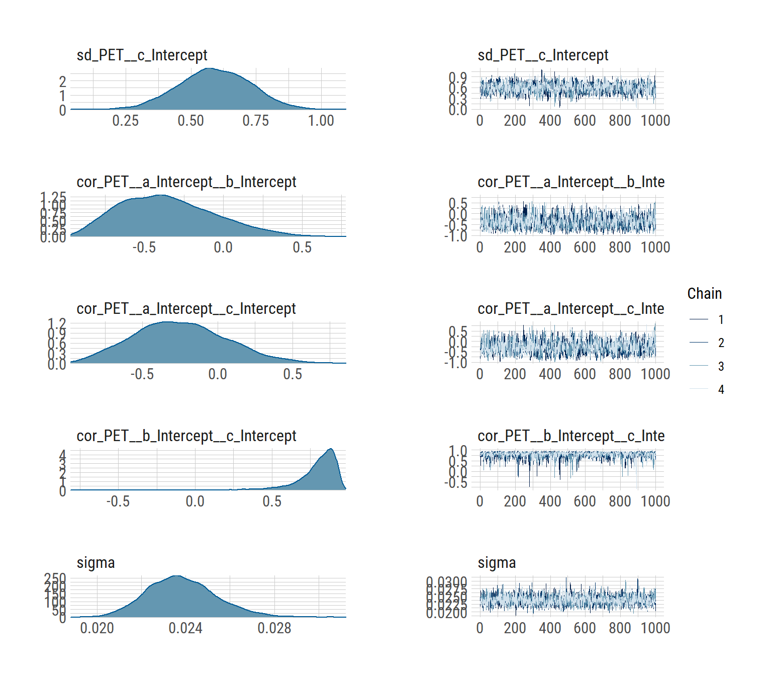
plot(hill_multilevelbayes_fit, ask = FALSE)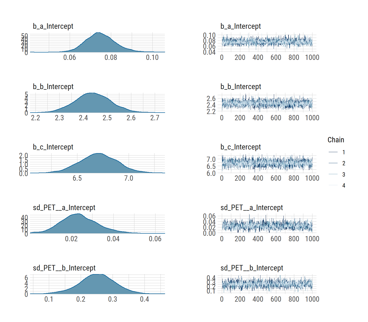
Fits
And let’s see the individual fits. Because we’ve defined a function, we first need to expose it, using the expose_functions command.
expose_functions(hill_multilevelbayes_fit, vectorize = TRUE)

hill_mlbayes_pred <- predict(hill_multilevelbayes_fit,
                             newdata=hill_predtimes) %>%
  as_tibble()
hill_mlbayes_fitted <- fitted(hill_multilevelbayes_fit,
                              newdata=hill_predtimes) %>%
  as_tibble()

hill_mlbayes_ribbons <- tibble(
  PET = hill_predtimes$PET,
  Time = hill_predtimes$Time,
  parentFraction = hill_mlbayes_fitted$Estimate,
  pred_lower = hill_mlbayes_pred$Q2.5,
  pred_upper = hill_mlbayes_pred$Q97.5,
  fitted_lower = hill_mlbayes_fitted$Q2.5,
  fitted_upper = hill_mlbayes_fitted$Q97.5)

ggplot(pf_modeldata, aes(x=Time, y=parentFraction)) +
  geom_point() +
  geom_line(data=hill_mlbayes_ribbons, aes(y=parentFraction), colour=colourcodes[3],
            size=1)  +
  geom_ribbon(data=hill_mlbayes_ribbons, alpha=0.2, aes(ymin=pred_lower,
                                                        ymax=pred_upper),
              fill=colourcodes[3]) +
  geom_ribbon(data=hill_mlbayes_ribbons, alpha=0.5, aes(ymin=fitted_lower,
                                                        ymax=fitted_upper),
              fill=colourcodes[3]) +
  facet_wrap(~PET, ncol=4)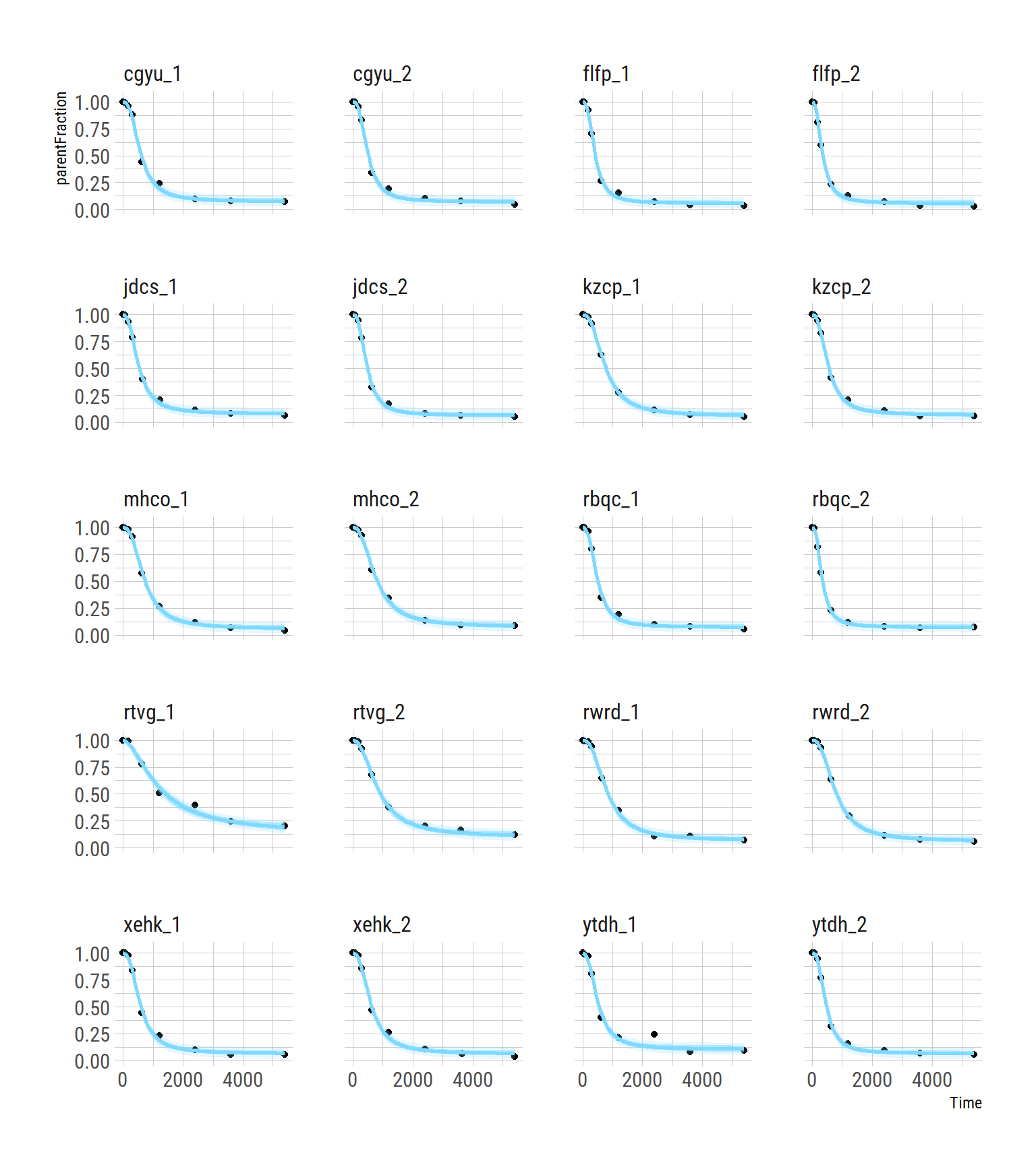
This is really illuminating to compare with the above single-subject plots: the inner blue ribbons contain the 95% credible interval, and the outer ones contain the 95% prediction intervals, and we can see that they’re pretty tight compared to the fitting of the single curve above. We also see that the ugly data point in the second to last curve falls well outside the 95% predicted interval, suggesting that the model believes that it was an unlikely observation.
The Average Curve
So, we’ve looked a little bit at the credible intervals, and the prediction intervals. I thought I’d take the opportunity to take a slightly closer look at the the average curve. Here, based on our model, we can examine four kinds of uncertainty around the average curve:
- Our model’s uncertainty around our estimate of the average curve at each given time point (fixed effects credible interval)
- The values our model would expect to observe from the average individual (based on measurement error etc.) (fixed effects prediction interval)
- Our model’s uncertainty around an estimate of the curve for a new individual, not yet examined, based on the remainder of the sample (fixed + random effects credible interval)
- The values our model would expect to observe from a new individual (based on measurement error + their not being “the average individual” etc.) (fixed + random effects prediction interval)
Let’s give it a go.
probnames <- c(20, 50, 80, 95)
probs <- c(40, 60, 25, 75, 10, 90, 2.5, 97.5)/100

probtitles <- probs[order(probs)]*100
probtitles <- paste("Q", probtitles, sep="")


hill_mlbayes_avgpred <- predict(hill_multilevelbayes_fit,
                             newdata=list(Time=hill_predtimes$Time),
                             re_formula = NA,
                             probs=probs) %>%
  as_tibble() %>%
  mutate(Curve = "Prediction Intervals",
         Effects = "Fixed")

hill_mlbayes_avgfitted <- fitted(hill_multilevelbayes_fit,
                             newdata=list(Time=hill_predtimes$Time),
                             re_formula = NA,
                             probs=probs) %>%
  as_tibble() %>%
  mutate(Curve = "Credible Intervals",
         Effects = "Fixed")

hill_mlbayes_avgfitted_ns <- fitted(hill_multilevelbayes_fit,
                             newdata=list(Time=hill_predtimes$Time,
                                          PET=rep("new", nrow(hill_predtimes))),
                             probs=probs, allow_new_levels=TRUE) %>%
  as_tibble() %>%
  mutate(Curve = "Credible Intervals",
         Effects = "Fixed + Random")

hill_mlbayes_avgpred_ns <- predict(hill_multilevelbayes_fit,
                             newdata=list(Time=hill_predtimes$Time,
                                          PET=rep("new", nrow(hill_predtimes))),
                             probs=probs, allow_new_levels=TRUE) %>%
  as_tibble() %>%
  mutate(Curve = "Prediction Intervals",
         Effects = "Fixed + Random")

hill_mlbayes_aribbons <- bind_rows(hill_mlbayes_avgpred,
                                   hill_mlbayes_avgfitted,
                                   hill_mlbayes_avgpred_ns,
                                   hill_mlbayes_avgfitted_ns) %>%
  mutate(Time = rep(hill_predtimes$Time, 4))
avg_pal <- viridis::plasma(n=4)
names(avg_pal) <- paste(probnames, "%", sep="")
ggplot(hill_mlbayes_aribbons, aes(x=Time, y=Estimate)) +
geom_ribbon(aes_string(ymin=probtitles[1], ymax=probtitles[2]),
fill=avg_pal[1], alpha=0.6) +
geom_ribbon(aes_string(ymin=probtitles[7], ymax=probtitles[8]),
fill=avg_pal[1], alpha=0.6) +
geom_ribbon(aes_string(ymin=probtitles[2], ymax=probtitles[3]),
fill=avg_pal[2], alpha=0.6) +
geom_ribbon(aes_string(ymin=probtitles[6], ymax=probtitles[7]),
fill=avg_pal[2], alpha=0.6) +
geom_ribbon(aes_string(ymin=probtitles[3], ymax=probtitles[4]),
fill=avg_pal[3], alpha=0.6) +
geom_ribbon(aes_string(ymin=probtitles[5], ymax=probtitles[6]),
fill=avg_pal[3], alpha=0.6) +
geom_ribbon(aes_string(ymin=probtitles[4], ymax=probtitles[5]),
fill=avg_pal[4], alpha=0.6) +
facet_wrap(Effects~Curve, ncol=2)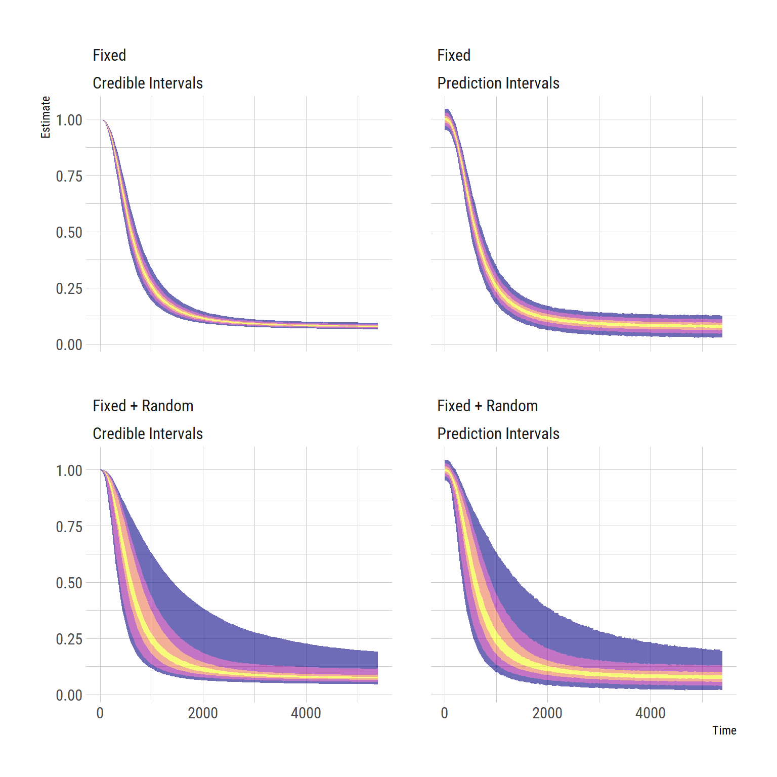
We can get quite a lot of information from these plots! We can see that we are quite certain of the average curve (top left), and that the amount of error around our curve, according to our model, is quite small (top right). We can also see that we could not hope to be able to use an average curve as a substitute for measuring the individual curves, because there is a lot of inter-individual variability (bottom left). The true inter-individual variability (bottom left) comprises the vast majority of the variance of the measured values, and the the additional measurement error constitutes a very small extra amount of variance (bottom right). We could also use the fixed+random prediction interval as a means by which to flag unlikely values during measurement, in case they have been entered incorrectly, or the machine is malfunctioning etc.
Comparing the Parameters and Fits
Parameters
Here we can compare the parameters from each of the methods to examine their shrinkage
hill_mlbayes_arrays <- coef(hill_multilevelbayes_fit)

hill_mlbayes_outcomes <- rbind(a=hill_mlbayes_arrays$PET[, , 1],
                                b=hill_mlbayes_arrays$PET[, , 2],
                                c=hill_mlbayes_arrays$PET[, , 3]) %>%
  as_tibble(rownames='PET') %>%
  mutate(Model = 'MCMC',
         Parameter = rep(c('a', 'b', 'c'), each=nrow(pfdata))) %>%
  select(PET, Parameter, Estimate, Model)

model_outcome_comparison <- bind_rows(nls_nlme_comparison, hill_mlbayes_outcomes)

ggplot(model_outcome_comparison, aes(x=Estimate, colour=Model, fill=Model)) +
  geom_density(alpha=0.3) +
  scale_fill_manual(values=colourpal) +
  scale_colour_manual(values=colourpal) +
  facet_wrap(~Parameter, scales="free")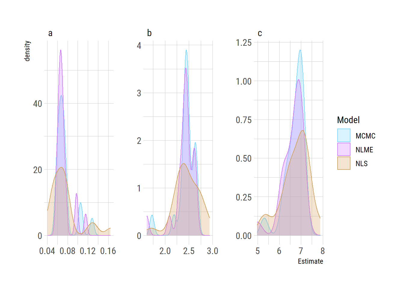
Here we can see the shrinkage of the parameters towards the respective means for the NLME and MCMC estimates.
Fits
Let’s also compare fits. I’ll do it with larger panels so we can look a bit more closely to see any differences.
preddata <- tibble(
  PET = hill_nlspreds$PET,
  Time = hill_nlspreds$Time,
  NLS = hill_nlspreds$.fitted,
  NLME = hill_nlmepreds$.fitted,
  MCMC = hill_mlbayes_fitted$Estimate
) %>%
  gather(Model, parentFraction, -PET, -Time) %>%
  mutate(Model = fct_inorder(Model)) %>%
  arrange(PET, Time, Model)
## Warning: attributes are not identical across measure variables;
## they will be droppedggplot(pf_modeldata, aes(x=Time, y=parentFraction)) +
geom_point() +
geom_line(data=preddata, aes(y=parentFraction, colour=Model),
size=0.7) +
facet_wrap(~PET, ncol=2) +
scale_colour_manual(values=colourpal)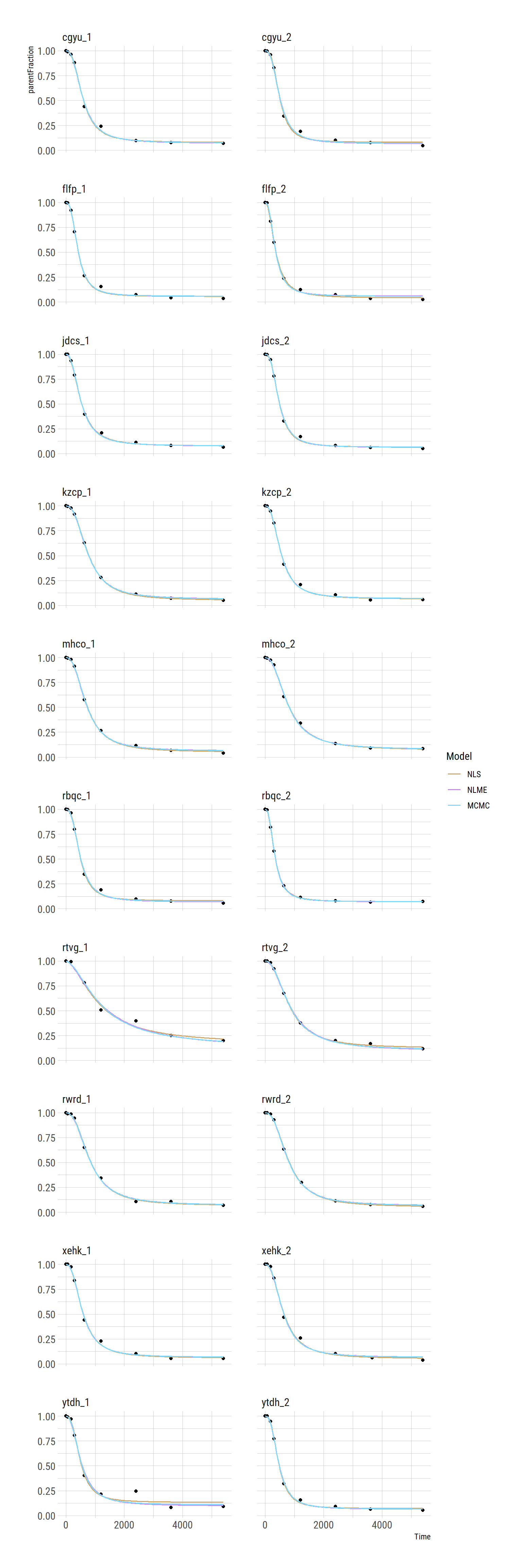
The curves are pretty close. We see that the second-to-last has the biggest deviations between methods, as we’d expect.
Conclusions
Here I’ve gone through how to perform nonlinear modelling using nonlinear least squares (NLS, using the minpack.lm and nls.multstart packages), multilevel maximum likelihood estimation (using the nlme package), and multilevel Bayesian modelling (using brms, which makes use of STAN). Of course it’s easiest to use the former, but we get the least information back, and are the most vulnerable to measurement error or inaccuracies in the data. Multilevel modelling allows us to take advantage of the similarities between individuals to derive better estimates. Using Bayesian methods, we can incorporate the knowledge that we already have based on previous experience, or previous studies, and gives us more information, and more flexibility. The Bayesian models require more thought though, and takes more computational resources.
I hope this has been helpful! I know it certainly has been for me, to be able to flick back to to copy the syntax and modify from when running these types of models in new scenarios.