TOC
Introduction
I wanted to do something different on this blog and go through something that’s less of my side-project, and more of my project-project, i.e. PET pharmacokinetic modelling. In Part 2, I’ll cover basic use of the kinfitr package and iteration.
The parts of this series are as follows:
If you want to mess around with these vignettes yourself without needing to install the package, you can fire up a binder containing everything by clicking the button below.
![]()
Packages
First, let’s load up our packages
#remotes::install_github("mathesong/kinfitr")

library(kinfitr)
library(tidyverse)
library(knitr)
library(cowplot)
library(mgcv)
library(ggforce)

theme_set(theme_light())
Reference Region Models
I’ll start off with a demonstration of how kinfitr can be used to fit reference region models, since they’re a little bit more straightforward. I will use the dataset included in the package, called simref. This dataset is simulated to correspond to data which can be successfully modelled with reversible reference-region approaches, with one-tissue dynamics in all regions (this is one of the assumptions of several reference tissue models. It doesn’t mean that there is no specific binding in a particular region, but it means that the transfer between compartments should equilibrate so quickly as to be possible to model it as the same compartment).
data(simref)Let’s have a look at how the data is structured:
head(simref)## # A tibble: 6 x 4
## Subjname PETNo PET tacs
## <chr> <dbl> <chr> <list>
## 1 hukw 1 hukw_1 <tibble [38 x 8]>
## 2 ybnx 1 ybnx_1 <tibble [38 x 8]>
## 3 olyl 1 olyl_1 <tibble [38 x 8]>
## 4 rocx 1 rocx_1 <tibble [38 x 8]>
## 5 gbiy 1 gbiy_1 <tibble [38 x 8]>
## 6 xsqz 1 xsqz_1 <tibble [38 x 8]>… and within the nested data under tacs is the following:
head(simref$tacs[[1]])## # A tibble: 6 x 8
## Times Reference ROI1 ROI2 ROI3 Weights StartTime Duration
## <dbl> <dbl> <dbl> <dbl> <dbl> <dbl> <dbl> <dbl>
## 1 0 0 0 0 0 0 0 0
## 2 0.567 0.137 0.203 0.0518 0.412 0.712 0.483 0.167
## 3 0.733 0.787 1.41 2.31 3.02 0.734 0.65 0.167
## 4 0.9 14.0 17.2 15.3 14.1 0.825 0.817 0.167
## 5 1.07 34.0 41.5 35.5 35.0 0.901 0.983 0.167
## 6 1.23 46.3 57.5 50.7 48.2 0.941 1.15 0.167Fitting the data
Fitting a single TAC
First let’s fit a single TAC to see how everything works. Here, I use the simplified reference tissue model. This model is quite flexible, though does have several assumptions (detailed really nicely here).
tacdata_1 <- simref$tacs[[1]]

t_tac <- tacdata_1$Times
reftac <- tacdata_1$Reference
roitac <- tacdata_1$ROI1
weights <- tacdata_1$Weights

fit1 <- srtm(t_tac, reftac, roitac)
Now let’s look at the fit
plot(fit1)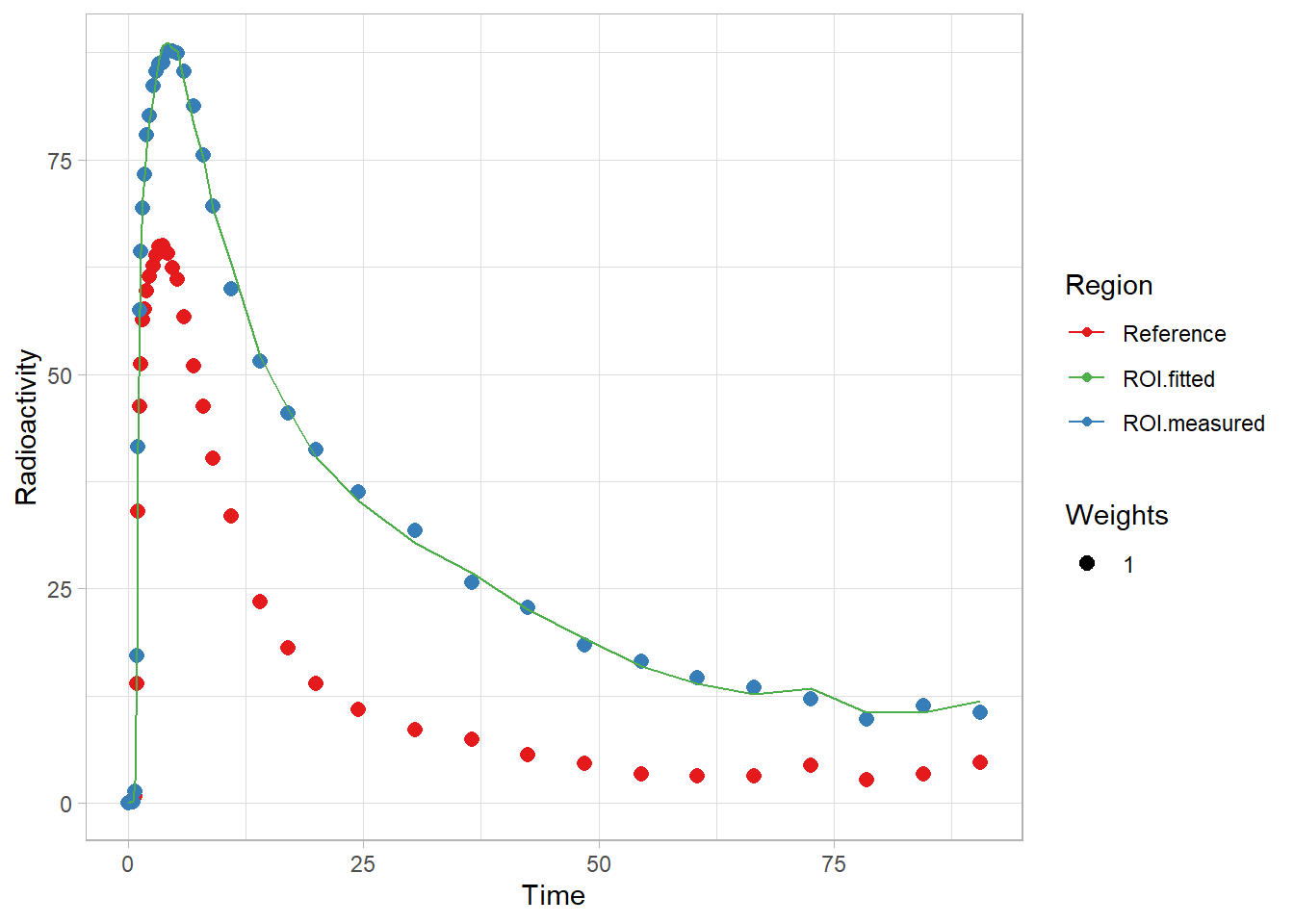
plot_residuals(fit1)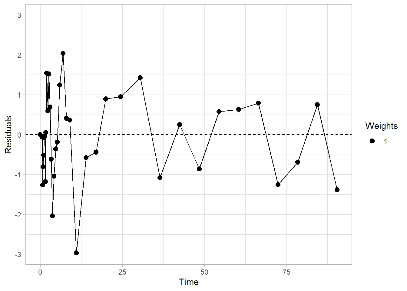
And what is in the fit object?
str(fit1)## List of 6
## $ par :'data.frame': 1 obs. of 3 variables:
## ..$ R1: num 1.23
## ..$ k2: num 0.102
## ..$ bp: num 1.49
## $ par.se :'data.frame': 1 obs. of 3 variables:
## ..$ R1.se: num 0.00499
## ..$ k2.se: num 0.0322
## ..$ bp.se: num 0.0199
## $ fit :List of 6
## ..$ m :List of 16
## .. ..$ resid :function ()
## .. ..$ fitted :function ()
## .. ..$ formula :function ()
## .. ..$ deviance :function ()
## .. ..$ lhs :function ()
## .. ..$ gradient :function ()
## .. ..$ conv :function ()
## .. ..$ incr :function ()
## .. ..$ setVarying:function (vary = rep(TRUE, length(useParams)))
## .. ..$ setPars :function (newPars)
## .. ..$ getPars :function ()
## .. ..$ getAllPars:function ()
## .. ..$ getEnv :function ()
## .. ..$ trace :function ()
## .. ..$ Rmat :function ()
## .. ..$ predict :function (newdata = list(), qr = FALSE)
## .. ..- attr(*, "class")= chr "nlsModel"
## ..$ convInfo:List of 5
## .. ..$ isConv : logi TRUE
## .. ..$ finIter : int 4
## .. ..$ finTol : num 1.49e-08
## .. ..$ stopCode : int 1
## .. ..$ stopMessage: chr "Relative error in the sum of squares is at most `ftol'."
## ..$ data : symbol modeldata
## ..$ call : language minpack.lm::nlsLM(formula = roitac ~ srtm_model(t_tac, reftac, R1, k2, bp), data = modeldata, start = start,| __truncated__ ...
## ..$ weights : num [1:38] 1 1 1 1 1 1 1 1 1 1 ...
## ..$ control :List of 9
## .. ..$ ftol : num 1.49e-08
## .. ..$ ptol : num 1.49e-08
## .. ..$ gtol : num 0
## .. ..$ diag : list()
## .. ..$ epsfcn : num 0
## .. ..$ factor : num 100
## .. ..$ maxfev : int(0)
## .. ..$ maxiter: num 200
## .. ..$ nprint : num 0
## ..- attr(*, "class")= chr "nls"
## $ weights: num [1:38] 1 1 1 1 1 1 1 1 1 1 ...
## $ tacs :'data.frame': 38 obs. of 4 variables:
## ..$ Time : num [1:38] 0 0.567 0.733 0.9 1.067 ...
## ..$ Reference : num [1:38] 0 0.137 0.787 13.964 34.008 ...
## ..$ Target : num [1:38] 0 0.203 1.413 17.179 41.503 ...
## ..$ Target_fitted: num [1:38] 1.81e-15 2.68e-01 2.68 1.80e+01 4.20e+01 ...
## $ model : chr "srtm"
## - attr(*, "class")= chr [1:2] "srtm" "kinfit"There’s a lot.
Of primary importance:
- par contains the fitted parameters. In this case, these parameters are R1 (\(=\frac{K_1}{K_1'}\)) and k2. This is what we’ll use most of all.
fit1$par## R1 k2 bp
## 1 1.233546 0.1016237 1.488339- par.se contains the standard errors as a fraction of the values
fit1$par.se## R1.se k2.se bp.se
## 1 0.004986278 0.03224267 0.01992612So here we can see that the parameters were estimated with a pretty high degree of certainty: 2% error on BPND is not bad at all!
- fit contains the actual model fit object, which we can do all sorts of great things with
- weights, tacs, model are pretty self-explanatory
The fit object being there means we can do all of the things that R, being a language designed by statisticians, allows us to do easily
g <- fit1$fit

coef(g)
## R1 k2 bp
## 1.2335455 0.1016237 1.4883389resid(g)## [1] -1.814790e-15 -6.503612e-02 -1.263658e+00 -8.041934e-01 -5.149457e-01
## [6] -7.244154e-02 -3.525757e-02 -1.183420e+00 5.159218e-02 1.539581e+00
## [11] 6.016639e-01 1.516351e+00 6.913366e-01 -6.188564e-01 -2.039015e+00
## [16] -1.046386e+00 -3.622996e-01 -1.916459e-01 1.242381e+00 2.035547e+00
## [21] 4.086986e-01 3.637660e-01 -2.969245e+00 -5.773616e-01 -4.389941e-01
## [26] 8.916004e-01 9.471013e-01 1.425524e+00 -1.081132e+00 2.508164e-01
## [31] -8.628823e-01 5.746597e-01 6.287208e-01 7.888887e-01 -1.258560e+00
## [36] -6.968996e-01 7.543217e-01 -1.383989e+00
## attr(,"label")
## [1] "Residuals"vcov(g)## R1 k2 bp
## R1 3.783235e-05 -1.085198e-05 3.109032e-05
## k2 -1.085198e-05 1.073623e-05 -5.748971e-05
## bp 3.109032e-05 -5.748971e-05 8.795270e-04AIC(g)## [1] 119.7931BIC(g)## [1] 126.3434Iterating Across Individuals for One Region
Now let’s fit a model to more TACs, one from each individual. I’ll also use a different model for fun (and because it’s faster): in this case MRTM1. MRTM1 is a linearised model, which estimates both BPND and k2’.
Note: Most linearised models have, as either a required or optional parameter, a t* value. I’ll cover this in another vignette. But, for now, we don’t need to worry about this as MRTM1 and MRTM2 require a t* value only in the case of not following 1-tissue compartment dynamics, and this data was specifically simulated to follow this. But I’ll use a value for some of the other models, but read the other vignette to understand how I came to choose these values.
simref <- simref %>%
  group_by(Subjname, PETNo) %>%
  mutate(MRTM1fit = map(tacs, ~mrtm1(t_tac = .x$Times, reftac = .x$Reference,
                                      roitac = .x$ROI1,
                                      weights = .x$Weights))) %>%
  ungroup()
Now let’s look at the distribution of our BPND values
simref <- simref %>%
  mutate(bp_MRTM1 = map_dbl(MRTM1fit, c("par", "bp")))

ggplot(simref, aes(x=bp_MRTM1)) +
  geom_histogram(fill="grey", colour="black", bins=10)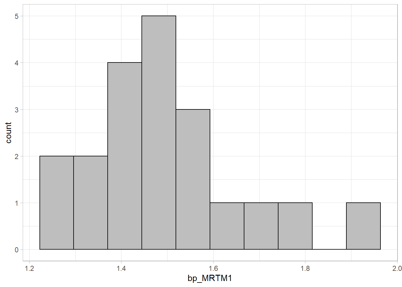
That looks fairly normal!
Iterating across Multiple Regions from Multiple Individuals
Now, let’s fit all the regions, and use a bunch of different models. First, though, we need to account for some extra requirements of some other models.
k2prime
One requirement of several linear reference region models is that a k2’ (k2 prime) value be specified, i.e. the rate of efflux from the reference region. The prime means that it is from the reference tissue. Note: this is not the same as k2: the assumption is that \(\frac{K_1}{k_2}=\frac{K_1'}{k_2'}\)). We can estimate a k2* value by fitting this value using one of the models which fits it. k2’ can be assessed using SRTM indirectly, using R1 and k2 (\(\frac{k_2}{R1}\)), or directly using MRTM1. It should, in theory, be stable across the brain, since it is a function of the reference region, and therefore it can be fitted for one region (usually selected as one with particularly low levels of noise) which we have already done above (or alternatively averaged over several regions). Let’s first extract the k2’ values into their own column first.
simref <- simref %>%
  mutate(k2prime = map_dbl(MRTM1fit, c("par", "k2prime")))

ggplot(simref, aes(x=k2prime)) +
  geom_histogram(fill="grey", colour="black", bins=10)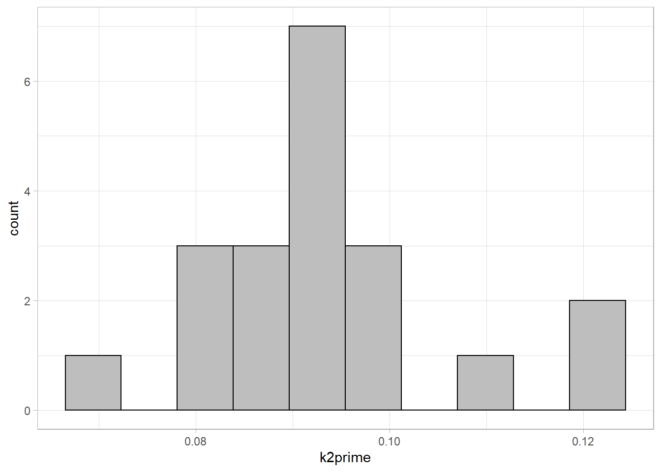
Model fitting
Now, we have extracted estimated k2prime values, and selected t* values. We are ready to fit most models.
First, we rearrange the data a little bit, so that it is chunked at the level of ROIs within regions, as opposed to individuals. Currently the data looks as follows:
simref <- simref %>%
  select(-MRTM1fit, -bp_MRTM1)

simref
## # A tibble: 20 x 5
## Subjname PETNo PET tacs k2prime
## <chr> <dbl> <chr> <list> <dbl>
## 1 hukw 1 hukw_1 <tibble [38 x 8]> 0.0825
## 2 ybnx 1 ybnx_1 <tibble [38 x 8]> 0.119
## 3 olyl 1 olyl_1 <tibble [38 x 8]> 0.0972
## 4 rocx 1 rocx_1 <tibble [38 x 8]> 0.0934
## 5 gbiy 1 gbiy_1 <tibble [38 x 8]> 0.101
## 6 xsqz 1 xsqz_1 <tibble [38 x 8]> 0.0923
## 7 rsop 1 rsop_1 <tibble [38 x 8]> 0.0910
## 8 hdzx 1 hdzx_1 <tibble [38 x 8]> 0.0990
## 9 ruam 1 ruam_1 <tibble [38 x 8]> 0.0782
## 10 tfig 1 tfig_1 <tibble [38 x 8]> 0.0949
## 11 dkkj 1 dkkj_1 <tibble [38 x 8]> 0.0911
## 12 ddgm 1 ddgm_1 <tibble [38 x 8]> 0.0851
## 13 gwbl 1 gwbl_1 <tibble [38 x 8]> 0.122
## 14 udof 1 udof_1 <tibble [38 x 8]> 0.0872
## 15 dtxj 1 dtxj_1 <tibble [38 x 8]> 0.0832
## 16 rcjh 1 rcjh_1 <tibble [38 x 8]> 0.0844
## 17 vlvv 1 vlvv_1 <tibble [38 x 8]> 0.0943
## 18 ultq 1 ultq_1 <tibble [38 x 8]> 0.0702
## 19 samf 1 samf_1 <tibble [38 x 8]> 0.110
## 20 jpjc 1 jpjc_1 <tibble [38 x 8]> 0.0928Next, we want to chunk at a different level. Instead of individuals, we want to chunk at regions of each individual.
simref_long <- simref %>%
  unnest(tacs) %>%
  select(-StartTime, -Duration, -PET)

simref_long
## # A tibble: 760 x 9
## Subjname PETNo Times Reference ROI1 ROI2 ROI3 Weights k2prime
## <chr> <dbl> <dbl> <dbl> <dbl> <dbl> <dbl> <dbl> <dbl>
## 1 hukw 1 0 0 0 0 0 0 0.0825
## 2 hukw 1 0.567 0.137 0.203 0.0518 0.412 0.712 0.0825
## 3 hukw 1 0.733 0.787 1.41 2.31 3.02 0.734 0.0825
## 4 hukw 1 0.9 14.0 17.2 15.3 14.1 0.825 0.0825
## 5 hukw 1 1.07 34.0 41.5 35.5 35.0 0.901 0.0825
## 6 hukw 1 1.23 46.3 57.5 50.7 48.2 0.941 0.0825
## 7 hukw 1 1.4 51.2 64.3 55.4 54.6 0.958 0.0825
## 8 hukw 1 1.57 56.3 69.4 59.9 58.2 0.970 0.0825
## 9 hukw 1 1.73 57.6 73.2 63.5 61.4 0.979 0.0825
## 10 hukw 1 1.98 59.7 77.9 66.4 64.5 0.988 0.0825
## # ... with 750 more rowsAnd now we make it into a very long format (i.e. 760 rows to 2280 rows).
simref_long <- simref_long %>%
  gather(key = Region, value = TAC, -Times, -Weights,
         -Subjname, -PETNo, -k2prime, -Reference)

simref_long
## # A tibble: 2,280 x 8
## Subjname PETNo Times Reference Weights k2prime Region TAC
## <chr> <dbl> <dbl> <dbl> <dbl> <dbl> <chr> <dbl>
## 1 hukw 1 0 0 0 0.0825 ROI1 0
## 2 hukw 1 0.567 0.137 0.712 0.0825 ROI1 0.203
## 3 hukw 1 0.733 0.787 0.734 0.0825 ROI1 1.41
## 4 hukw 1 0.9 14.0 0.825 0.0825 ROI1 17.2
## 5 hukw 1 1.07 34.0 0.901 0.0825 ROI1 41.5
## 6 hukw 1 1.23 46.3 0.941 0.0825 ROI1 57.5
## 7 hukw 1 1.4 51.2 0.958 0.0825 ROI1 64.3
## 8 hukw 1 1.57 56.3 0.970 0.0825 ROI1 69.4
## 9 hukw 1 1.73 57.6 0.979 0.0825 ROI1 73.2
## 10 hukw 1 1.98 59.7 0.988 0.0825 ROI1 77.9
## # ... with 2,270 more rowsAnd now we nest it again, with our desired level of chunking.
simref_long <- simref_long %>%
  group_by(Subjname, PETNo, k2prime, Region) %>%
  nest(tacdata = -c(Subjname, PETNo, k2prime, Region))

simref_long
## # A tibble: 60 x 5
## # Groups: Subjname, PETNo, k2prime, Region [60]
## Subjname PETNo k2prime Region tacdata
## <chr> <dbl> <dbl> <chr> <list>
## 1 hukw 1 0.0825 ROI1 <tibble [38 x 4]>
## 2 ybnx 1 0.119 ROI1 <tibble [38 x 4]>
## 3 olyl 1 0.0972 ROI1 <tibble [38 x 4]>
## 4 rocx 1 0.0934 ROI1 <tibble [38 x 4]>
## 5 gbiy 1 0.101 ROI1 <tibble [38 x 4]>
## 6 xsqz 1 0.0923 ROI1 <tibble [38 x 4]>
## 7 rsop 1 0.0910 ROI1 <tibble [38 x 4]>
## 8 hdzx 1 0.0990 ROI1 <tibble [38 x 4]>
## 9 ruam 1 0.0782 ROI1 <tibble [38 x 4]>
## 10 tfig 1 0.0949 ROI1 <tibble [38 x 4]>
## # ... with 50 more rowsAnd within each chunk is the following:
simref_long$tacdata[[1]]## # A tibble: 38 x 4
## Times Reference Weights TAC
## <dbl> <dbl> <dbl> <dbl>
## 1 0 0 0 0
## 2 0.567 0.137 0.712 0.203
## 3 0.733 0.787 0.734 1.41
## 4 0.9 14.0 0.825 17.2
## 5 1.07 34.0 0.901 41.5
## 6 1.23 46.3 0.941 57.5
## 7 1.4 51.2 0.958 64.3
## 8 1.57 56.3 0.970 69.4
## 9 1.73 57.6 0.979 73.2
## 10 1.98 59.7 0.988 77.9
## # ... with 28 more rowsNow we can proceed to fitting models to all the regions.
simref_long <- simref_long %>%
  group_by(Subjname, PETNo, Region) %>%

  # SRTM
  mutate(SRTM = map(tacdata,
                         ~srtm(t_tac=.x$Times, reftac = .x$Reference,
                               roitac = .x$TAC,
                               weights = .x$Weights)),
         SRTM = map_dbl(SRTM, c("par", "bp"))) %>%

  # MRTM1
  mutate(MRTM1 = map(tacdata,
                         ~mrtm1(t_tac=.x$Times, reftac = .x$Reference,
                               roitac = .x$TAC,
                               weights = .x$Weights)),
         MRTM1 = map_dbl(MRTM1, c("par", "bp"))) %>%

  # MRTM2
  mutate(MRTM2 = map2(tacdata, k2prime,
                         ~mrtm2(t_tac=.x$Times, reftac = .x$Reference,
                               roitac = .x$TAC, k2prime = .y,
                               weights = .x$Weights)),
         MRTM2 = map_dbl(MRTM2, c("par", "bp"))) %>%

  # refLogan
  mutate(refLogan = map2(tacdata, k2prime,
                         ~refLogan(t_tac=.x$Times, reftac = .x$Reference,
                               roitac = .x$TAC, k2prime = .y,
                               weights = .x$Weights, tstarIncludedFrames = 10)),
         refLogan = map_dbl(refLogan, c("par", "bp"))) %>%

  # refmlLogan
  mutate(refmlLogan = map2(tacdata, k2prime,
                         ~refmlLogan(t_tac=.x$Times, reftac = .x$Reference,
                               roitac = .x$TAC, k2prime = .y,
                               weights = .x$Weights, tstarIncludedFrames = 10)),
         refmlLogan = map_dbl(refmlLogan, c("par", "bp"))) %>%
  ungroup()
Comparisons between Models
Now let’s check the correlations between the estimated BPND values.
simref_bpvals <- simref_long %>%
  ungroup() %>%
  select(Region, SRTM, refLogan, refmlLogan, MRTM1, MRTM2)

refvals <- ggplot(simref_bpvals, aes(x = .panel_x, y = .panel_y,
                                     colour=Region, fill=Region)) +
                      geom_point(position = 'auto') +
                      geom_autodensity(alpha = 0.3, colour = NA,
                                       position = 'identity') +
                      facet_matrix(vars(SRTM, refLogan, refmlLogan,
                                        MRTM1, MRTM2),
                                   layer.diag = 2) +
                      geom_smooth(method="lm", se=F) +
                      guides(colour=FALSE, fill=FALSE)

print(refvals)
## `geom_smooth()` using formula 'y ~ x'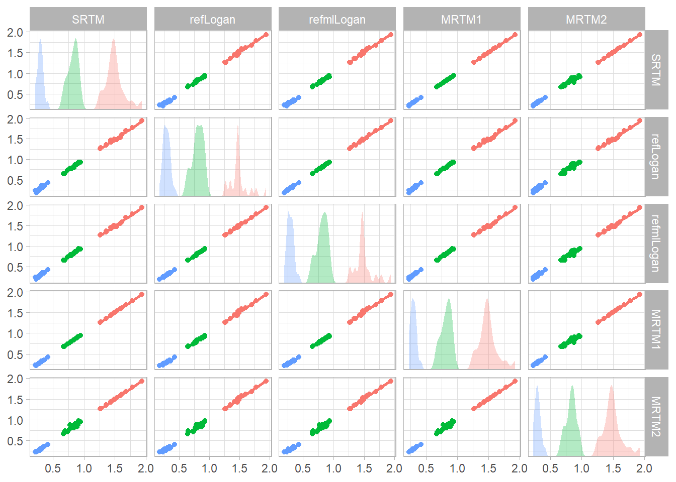
rm(simref_long) # Removing to free up some memoryArterial Input Models
Now we will work with some data for which there is no reference region. This is data collected using [\({11}\)C]PBR28, which binds to the 18kDa translocator protein, which is found throughout the brain, meaning that there is no reference region.
Some of the models here take a little while to run, so I’ll cut the dataset short to 4 PET measurements.
Blood Processing
The first, complicated aspect of working with data for which we must use the arterial plasma as a reference is that the blood data is collected through a parallel data collection, and is stored separately. I’ve written up another vignette about how to do this. But, for expedience, here I’ll just interpolate some data which was already processed. Let’s look at how the data looks, and what’s in the processed blood data for a random subject.
data(pbr28)

pbr28 <- pbr28[1:4,]

names(pbr28)
## [1] "PET" "Subjname" "PETNo" "tacs" "procblood" "input"
## [7] "Genotype" "injRad" "petinfo" "blooddata" "tactimes"head(pbr28$procblood[[2]])## # A tibble: 6 x 3
## Time Cbl_dispcorr Cpl_metabcorr
## <dbl> <dbl> <dbl>
## 1 0 0 0
## 2 1 0.0150 0.0232
## 3 2 0.0300 0.0464
## 4 3 0.0449 0.0696
## 5 4 0.0599 0.0928
## 6 5 0.0749 0.116Here, we were provided with Time (in seconds), the radioactivity in blood after dispersion correction, and the radioactivity in plasma after metabolite correction. We want to turn this data into an “input” object: arranged with all the things we need for modelling. Of note, because the plasma has already been metabolite-corrected, we will set the parent fraction to 1 throughout (since, in the given plasma values, the parent fraction is 100%), since we don’t want the function correcting for metabolites again. Once again, check out the blood processing vignette if you want to know more about blood processing in general.
If we wanted to process the blood data for one subject:
input <- blood_interp(
  t_blood = pbr28$procblood[[2]]$Time / 60,
  blood = pbr28$procblood[[2]]$Cbl_dispcorr,
  t_plasma = pbr28$procblood[[2]]$Time / 60,
  plasma = pbr28$procblood[[2]]$Cpl_metabcorr,
  t_parentfrac = 1, parentfrac = 1
)

round(head(input), 2)
## # A tibble: 6 x 5
## Time Blood Plasma ParentFraction AIF
## <dbl> <dbl> <dbl> <dbl> <dbl>
## 1 0 0 0 1 0
## 2 0.01 0.01 0.02 1 0.02
## 3 0.03 0.03 0.04 1 0.04
## 4 0.04 0.04 0.06 1 0.06
## 5 0.06 0.05 0.08 1 0.08
## 6 0.07 0.07 0.1 1 0.1Now, let’s do it for everyone.
pbr28 <- pbr28 %>%
  group_by(PET) %>%
  mutate(input = map(procblood,
                     ~blood_interp(
                        t_blood = .x$Time / 60,
                        blood = .x$Cbl_dispcorr,
                        t_plasma = .x$Time / 60,
                        plasma = .x$Cpl_metabcorr,
                        t_parentfrac = 1, parentfrac = 1))) %>%
  ungroup()
Great! Now we have input objects for each measurement.
Preparations for Modelling the TACs
Modelling the Delay
When it comes to modelling the TACs, the first thing we need to do is to match the timing of the TAC and the blood, by estimating the delay between the blood samples and the TAC. We can do this using one of the tissue compartmental models, with an additional parameter representing the delay. This is fitted by default if not specified in the nonlinear models, and will give an error if not specified in the other models.
pbr28 <- pbr28 %>%
  group_by(Subjname) %>%
  mutate(delayFit = map2(tacs, input,
                         ~twotcm(t_tac = .x$Times/60, # sec to min
                                 tac = .x$WB,
                                 input = .y,
                                 weights = .x$Weights,
                                 vB=0.05)))
## Warning: Problem with `mutate()` input `delayFit`.
## i
## Fitted parameters are hitting upper or lower limit bounds. Consider
## either modifying the upper and lower limit boundaries, or else using
## multstart when fitting the model (see the function documentation).
##
## i Input `delayFit` is `map2(...)`.
## i The error occurred in group 1: Subjname = "cgyu".## Warning in twotcm(t_tac = .x$Times/60, tac = .x$WB, input = .y, weights = .x$Weights, :
## Fitted parameters are hitting upper or lower limit bounds. Consider
## either modifying the upper and lower limit boundaries, or else using
## multstart when fitting the model (see the function documentation).## Warning: Problem with `mutate()` input `delayFit`.
## i
## Fitted parameters are hitting upper or lower limit bounds. Consider
## either modifying the upper and lower limit boundaries, or else using
## multstart when fitting the model (see the function documentation).
##
## i Input `delayFit` is `map2(...)`.
## i The error occurred in group 2: Subjname = "flfp".## Warning in twotcm(t_tac = .x$Times/60, tac = .x$WB, input = .y, weights = .x$Weights, :
## Fitted parameters are hitting upper or lower limit bounds. Consider
## either modifying the upper and lower limit boundaries, or else using
## multstart when fitting the model (see the function documentation).Let’s ignore the warnings for now. Not important at this point.
Now let’s check them, because delay fitting can go slightly awry.
walk2(pbr28$delayFit, pbr28$PET ,
      ~print(plot_inptac_fit(.x) + ggtitle(.y)))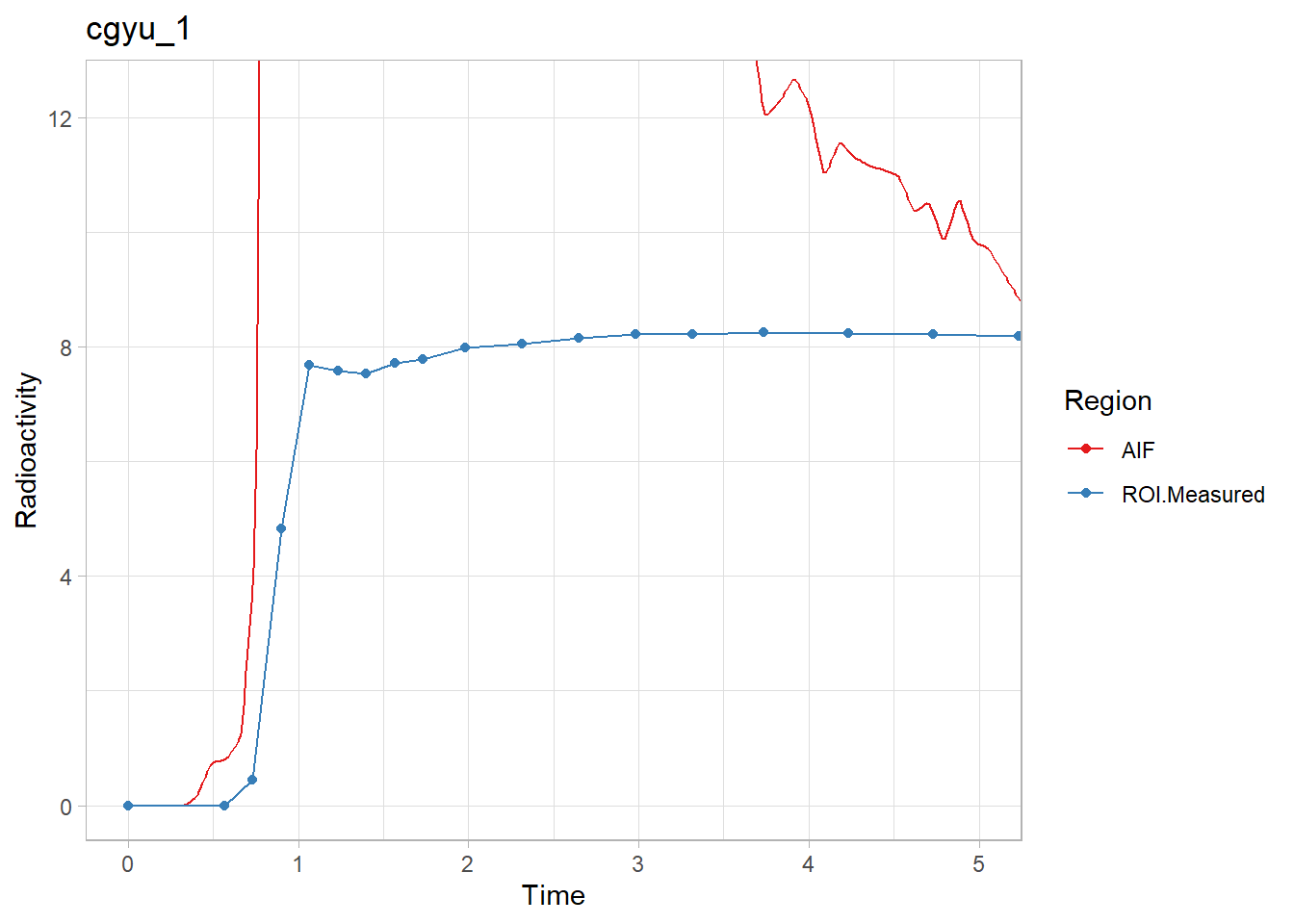
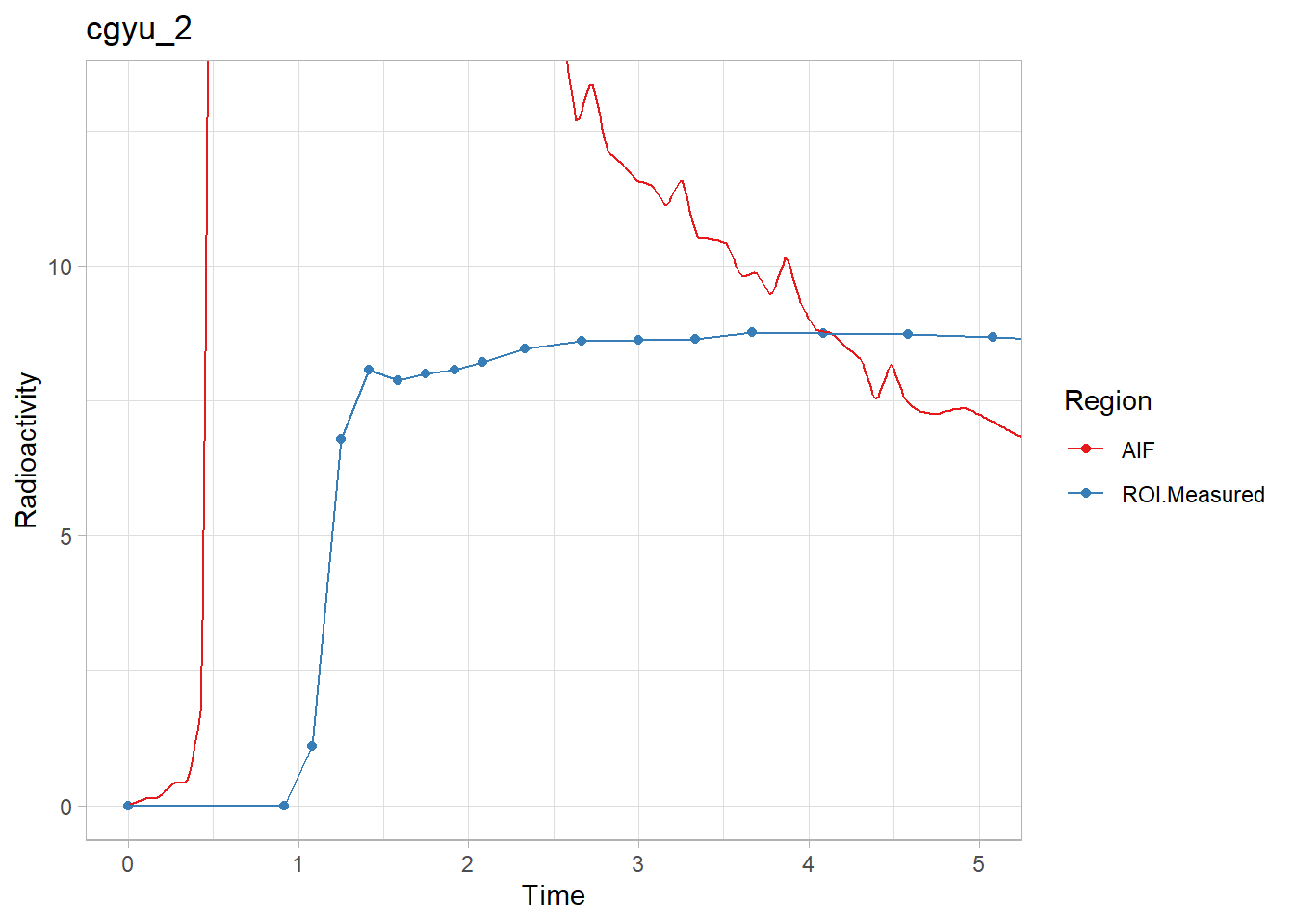
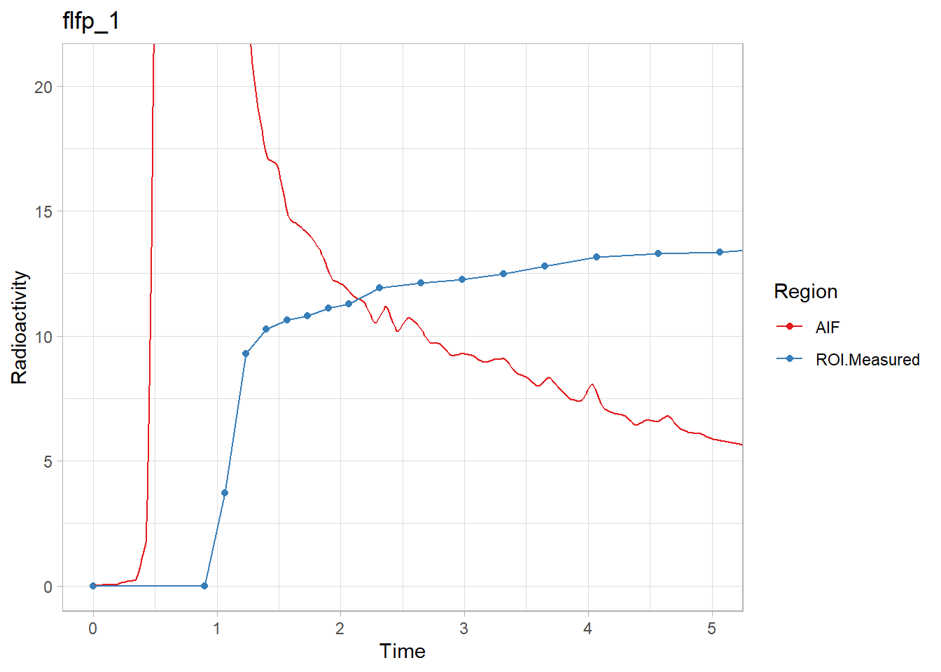
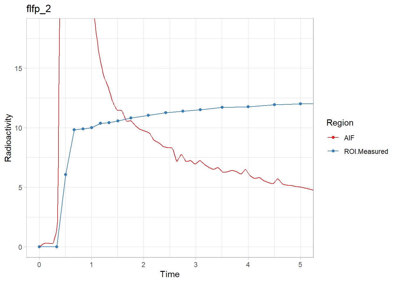
Hmmm… While the first and last look ok, the other two don’t look great. Let’s instead use only the first 10 minutes of the TACs to make sure we home in on the delay. Firstly, how many frames for 10 minutes?
which( pbr28$tacs[[1]]$Times/60 < 10)## [1] 1 2 3 4 5 6 7 8 9 10 11 12 13 14 15 16 17 18 19 20 21 22Ok, so let’s use 22 frames. We do this using the frameStartEnd parameter.
pbr28 <- pbr28 %>%
  group_by(Subjname) %>%
  mutate(delayFit = map2(tacs, input,
                         ~twotcm(t_tac = .x$Times/60, # sec to min
                                 tac = .x$WB,
                                 input = .y,
                                 weights = .x$Weights,
                                 vB=0.05,
                                 frameStartEnd = c(1, 22))))
## Warning: Problem with `mutate()` input `delayFit`.
## i
## Fitted parameters are hitting upper or lower limit bounds. Consider
## either modifying the upper and lower limit boundaries, or else using
## multstart when fitting the model (see the function documentation).
##
## i Input `delayFit` is `map2(...)`.
## i The error occurred in group 1: Subjname = "cgyu".## Warning in twotcm(t_tac = .x$Times/60, tac = .x$WB, input = .y, weights = .x$Weights, :
## Fitted parameters are hitting upper or lower limit bounds. Consider
## either modifying the upper and lower limit boundaries, or else using
## multstart when fitting the model (see the function documentation).## Warning: Problem with `mutate()` input `delayFit`.
## i
## Fitted parameters are hitting upper or lower limit bounds. Consider
## either modifying the upper and lower limit boundaries, or else using
## multstart when fitting the model (see the function documentation).
##
## i Input `delayFit` is `map2(...)`.
## i The error occurred in group 2: Subjname = "flfp".## Warning in twotcm(t_tac = .x$Times/60, tac = .x$WB, input = .y, weights = .x$Weights, :
## Fitted parameters are hitting upper or lower limit bounds. Consider
## either modifying the upper and lower limit boundaries, or else using
## multstart when fitting the model (see the function documentation).We can continue to ignore the warnings.
Now let’s check them again.
walk2(pbr28$delayFit, pbr28$PET ,
      ~print(plot_inptac_fit(.x) + ggtitle(.y)))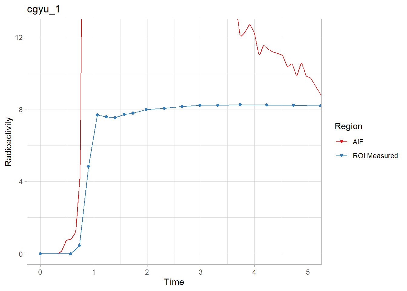
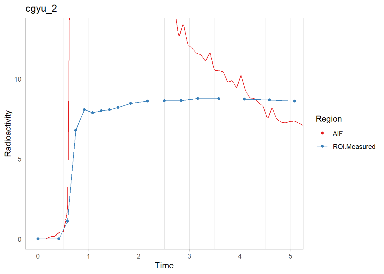
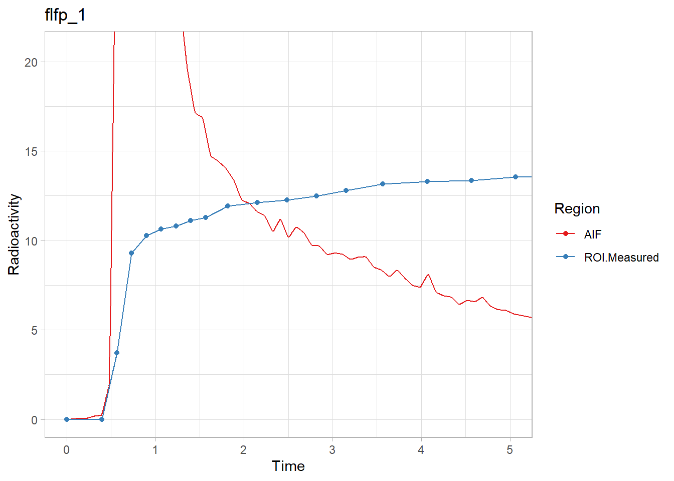

Beautiful! Now we’ll extract the delay values and use those in future models.
pbr28 <- pbr28 %>%
  group_by(Subjname) %>%
  mutate(inpshift = map_dbl(delayFit, c("par", "inpshift")))
Estimating t*
For the linear models, we will need to decide on t* values again. Instead of doing it again in this tutorial, we will just use 10 frames. I promise this works, but read more about it if you’re interested/skeptical.
Model Fitting
Now that we have interpolated the blood, modelled the delay and selected t* values, we are ready to start modelling the TACs. Let’s first select three TACs per individual.
pbr28 <- pbr28 %>%
  group_by(PET) %>%
  mutate(tacs = map(tacs, ~select(.x, Times, Weights, FC, STR, CBL))) %>%
  select(PET, tacs, input, inpshift)
Now we have to rearrange the data as before, but now we also have the input data. Let’s first separate the data, rearrange, and then join them again.
pbr28_input <- select(pbr28, PET, input)

pbr28_tacs <- select(pbr28, PET, tacs, inpshift)

pbr28_long <- pbr28_tacs %>%
  unnest(cols = tacs) %>%
  gather(key = Region, value = TAC, -Times, -Weights, -inpshift, -PET) %>%
  group_by(PET, inpshift, Region) %>%
  nest(tacdata = -c(PET, inpshift, Region)) %>%
  full_join(pbr28_input)
## Joining, by = "PET"And now let’s see what it looks like now.
pbr28_long## # A tibble: 12 x 5
## # Groups: PET, inpshift, Region [12]
## PET inpshift Region tacdata input
## <chr> <dbl> <chr> <list> <list>
## 1 cgyu_1 0.0497 FC <tibble [38 x 3]> <tibble [6,000 x 5]>
## 2 cgyu_2 0.153 FC <tibble [38 x 3]> <tibble [6,000 x 5]>
## 3 flfp_1 0.0458 FC <tibble [38 x 3]> <tibble [6,000 x 5]>
## 4 flfp_2 -0.00676 FC <tibble [38 x 3]> <tibble [6,000 x 5]>
## 5 cgyu_1 0.0497 STR <tibble [38 x 3]> <tibble [6,000 x 5]>
## 6 cgyu_2 0.153 STR <tibble [38 x 3]> <tibble [6,000 x 5]>
## 7 flfp_1 0.0458 STR <tibble [38 x 3]> <tibble [6,000 x 5]>
## 8 flfp_2 -0.00676 STR <tibble [38 x 3]> <tibble [6,000 x 5]>
## 9 cgyu_1 0.0497 CBL <tibble [38 x 3]> <tibble [6,000 x 5]>
## 10 cgyu_2 0.153 CBL <tibble [38 x 3]> <tibble [6,000 x 5]>
## 11 flfp_1 0.0458 CBL <tibble [38 x 3]> <tibble [6,000 x 5]>
## 12 flfp_2 -0.00676 CBL <tibble [38 x 3]> <tibble [6,000 x 5]>Now we can proceed to fitting models to all the regions. Let’s first just fit data for a single individual to see how it works, before iterating to show the general principle. Here, by not specifying vB (the blood volume fraction), it is also fitted. It’s usually about 5%, but as a modeller, one can choose to fit it, or set it. This is what we use the blood radioactivity for, and we subtract the contribution of blood containing radioactivity which has not crossed the blood-brain-barrier from the measured radioactivity in the region.
t_tac     <- pbr28_long$tacdata[[2]]$Times/60
tac       <- pbr28_long$tacdata[[2]]$TAC
input     <- pbr28_long$input[[2]]
weights   <- pbr28_long$tacdata[[2]]$Weights
inpshift  <- pbr28_long$inpshift[2]

pbrfit <- twotcm(t_tac, tac, input, weights, inpshift)

plot(pbrfit)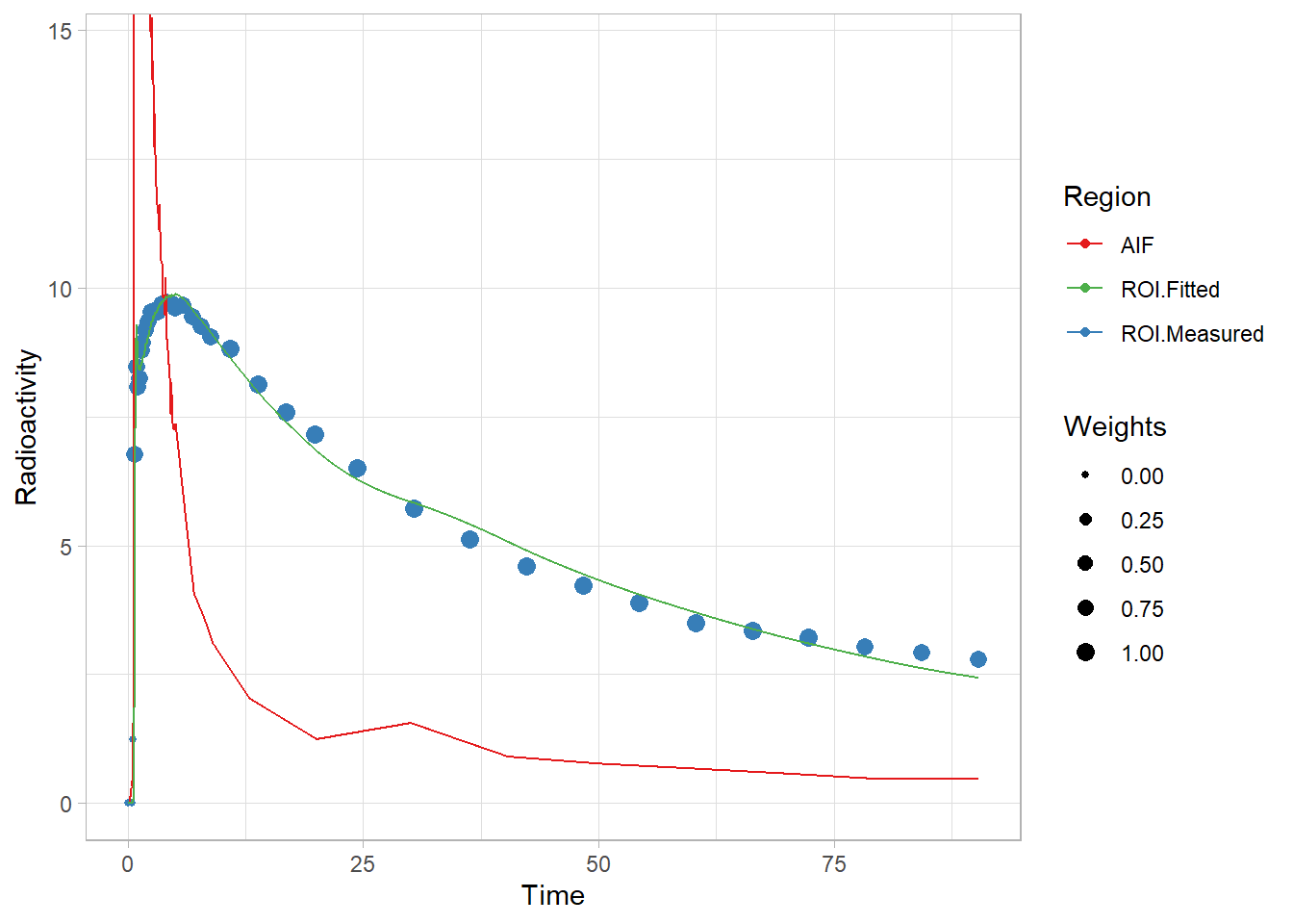
That fit looks ok! Not the greatest, but not too terrible. And let’s see what’s in the fit object.
str(pbrfit)## List of 9
## $ par :'data.frame': 1 obs. of 7 variables:
## ..$ K1 : num 0.113
## ..$ k2 : num 0.0925
## ..$ k3 : num 0.0525
## ..$ k4 : num 0.0521
## ..$ vB : num 0.057
## ..$ inpshift: num 0.153
## ..$ Vt : num 2.45
## $ par.se :'data.frame': 1 obs. of 7 variables:
## ..$ K1.se : num 0.022
## ..$ k2.se : num 0.12
## ..$ k3.se : num 0.339
## ..$ k4.se : num 0.198
## ..$ vB.se : num 0.0442
## ..$ inpshift.se: num 0
## ..$ Vt.se : num 0.0278
## $ fit :List of 6
## ..$ m :List of 16
## .. ..$ resid :function ()
## .. ..$ fitted :function ()
## .. ..$ formula :function ()
## .. ..$ deviance :function ()
## .. ..$ lhs :function ()
## .. ..$ gradient :function ()
## .. ..$ conv :function ()
## .. ..$ incr :function ()
## .. ..$ setVarying:function (vary = rep(TRUE, length(useParams)))
## .. ..$ setPars :function (newPars)
## .. ..$ getPars :function ()
## .. ..$ getAllPars:function ()
## .. ..$ getEnv :function ()
## .. ..$ trace :function ()
## .. ..$ Rmat :function ()
## .. ..$ predict :function (newdata = list(), qr = FALSE)
## .. ..- attr(*, "class")= chr "nlsModel"
## ..$ convInfo:List of 5
## .. ..$ isConv : logi TRUE
## .. ..$ finIter : int 13
## .. ..$ finTol : num 1.49e-08
## .. ..$ stopCode : int 1
## .. ..$ stopMessage: chr "Relative error in the sum of squares is at most `ftol'."
## ..$ data : symbol modeldata
## ..$ call : language minpack.lm::nlsLM(formula = tac ~ twotcm_model(t_tac, input, K1, k2, k3, k4, vB), data = modeldata, start = | __truncated__ ...
## ..$ weights : num [1:38] 0 0 0 0.896 0.896 ...
## ..$ control :List of 9
## .. ..$ ftol : num 1.49e-08
## .. ..$ ptol : num 1.49e-08
## .. ..$ gtol : num 0
## .. ..$ diag : list()
## .. ..$ epsfcn : num 0
## .. ..$ factor : num 100
## .. ..$ maxfev : int(0)
## .. ..$ maxiter: num 200
## .. ..$ nprint : num 0
## ..- attr(*, "class")= chr "nls"
## $ tacs :'data.frame': 38 obs. of 3 variables:
## ..$ Time : num [1:38] 0 0.417 0.583 0.75 0.917 ...
## ..$ Target : num [1:38] 0.00 7.90e-07 1.23 6.76 8.47 ...
## ..$ Target_fitted: num [1:38] -1.17e-14 1.97e-02 9.60e-02 5.81 9.19 ...
## $ input : tibble [6,000 x 5] (S3: interpblood/tbl_df/tbl/data.frame)
## ..$ Time : num [1:6000] 0 0.0151 0.0301 0.0452 0.0602 ...
## ..$ Blood : num [1:6000] 0 0 0 0 0 0 0 0 0 0 ...
## ..$ Plasma : num [1:6000] 0 0 0 0 0 0 0 0 0 0 ...
## ..$ ParentFraction: num [1:6000] 1 1 1 1 1 1 1 1 1 1 ...
## ..$ AIF : num [1:6000] 0 0 0 0 0 0 0 0 0 0 ...
## $ weights : num [1:38] 0 0 0 0.896 0.896 ...
## $ inpshift_fitted: logi FALSE
## $ vB_fitted : logi TRUE
## $ model : chr "2tcm"
## - attr(*, "class")= chr [1:2] "2tcm" "kinfit"You will notice that I’ve included, for example, the whole input object in the fit output. This is because this is the input (and TAC) after being time-shifted to match one another. This process is more complicated than it may seem, since it requires a fresh interpolation, sometimes padding the curves with values on either side. It’s very helpful for looking into poor fits, and diagnosing what’s going wrong. But it’s a bit of a memory hog. I advise some degree of caution with saving millions of model fits with arterial models. A good approach is to check the fits, and then extract only the parameters of interest for further analysis.
Another point worth making is with regards to the parameters
round(pbrfit$par, 3)## K1 k2 k3 k4 vB inpshift Vt
## 1 0.113 0.093 0.052 0.052 0.057 0.153 2.452round(pbrfit$par.se, 3)## K1.se k2.se k3.se k4.se vB.se inpshift.se Vt.se
## 1 0.022 0.12 0.339 0.198 0.044 0 0.028You will notice that the rate constants individually (often called the microparameters) are estimated with rather poor identifiability (i.e. high percentage standard error). However, their combination in VT (\(V_{T-2TCM}=\frac{K_1}{k_2}(1 + \frac{k_3}{k_4})\)) (often called a macroparameter) is much more identifiable. This is because the rate constants are highly dependent upon one another. So we should be careful about reading too much into their individual values, but we can derive much more value from VT. This is discussed more in the first post about the theory of PET modelling.
Let’s also just demonstrate a couple of other models and their fits. For the 2TCM1k, I’ll set vB to 0.05: this was the recommendation of the creator of this model, as it becomes rather unstable with so many parameters.
plot(onetcm(t_tac, tac, input, weights, inpshift)) +
       labs(title="1TCM",
            subtitle="Too few parameters, and underfits")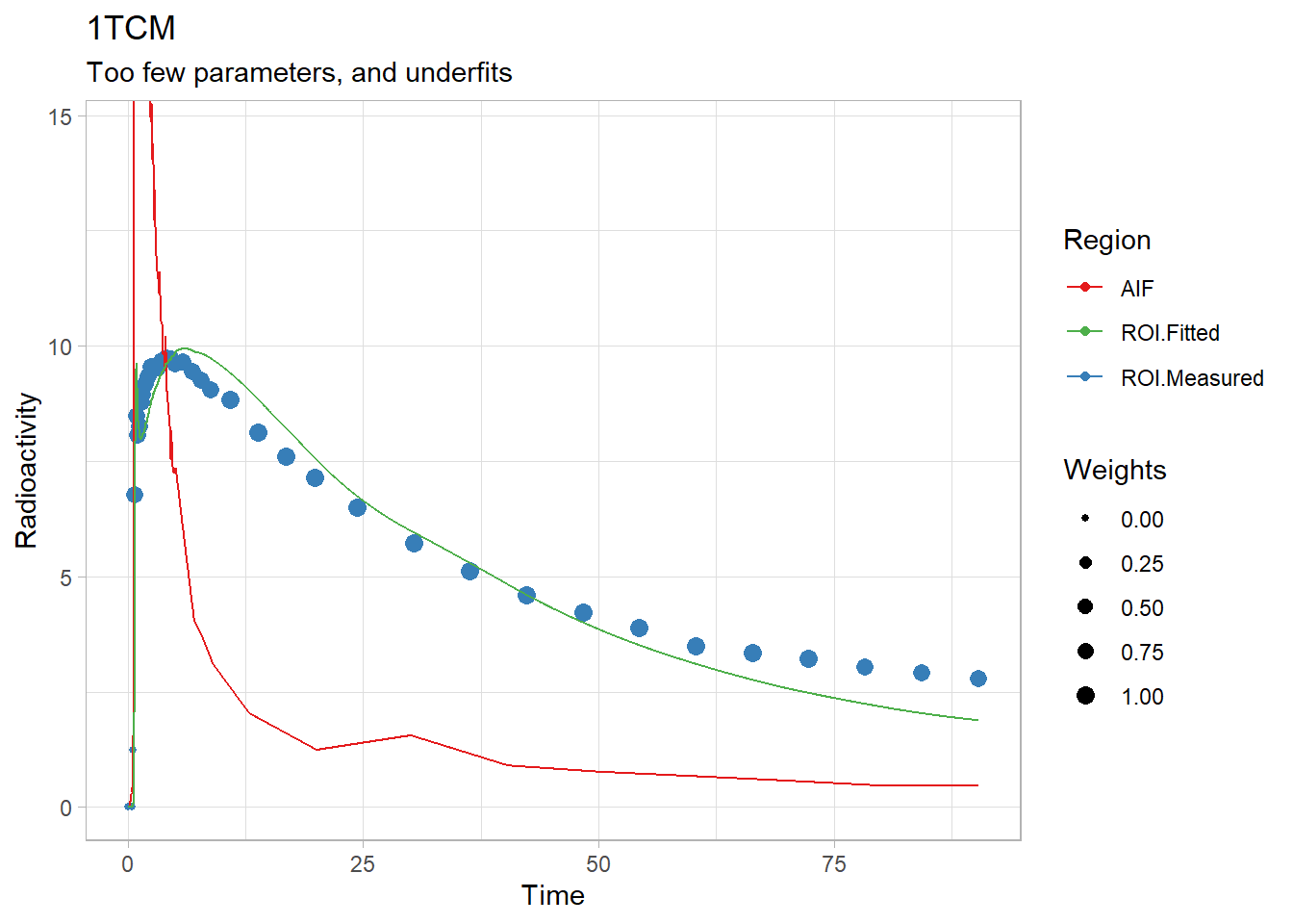
plot(twotcm1k(t_tac, tac, input, weights, inpshift, vB = 0.05)) +
       labs(title="2TCM1k",
            subtitle="Great fit, but macroparameters are less stable due to many parameters")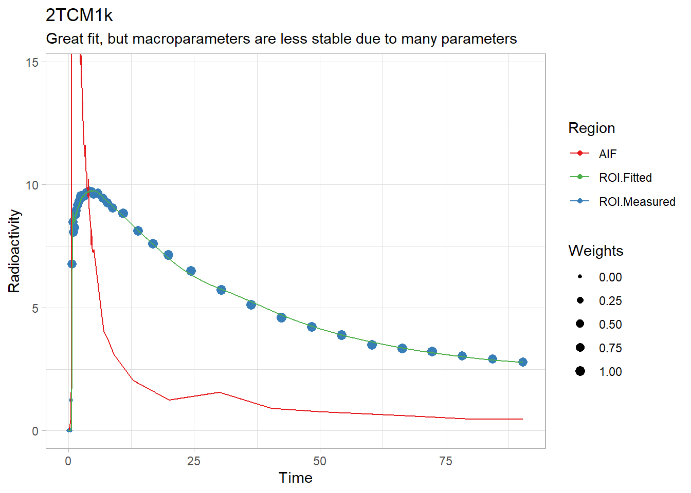
plot(Loganplot(t_tac, tac, input,
               tstarIncludedFrames =  10,
               weights, inpshift)) +
       labs(title="Logan Plot",
            subtitle="Linearised model using transformed data on both axes, after t* (10 frames)")
## Warning: Removed 2 rows containing missing values (geom_point).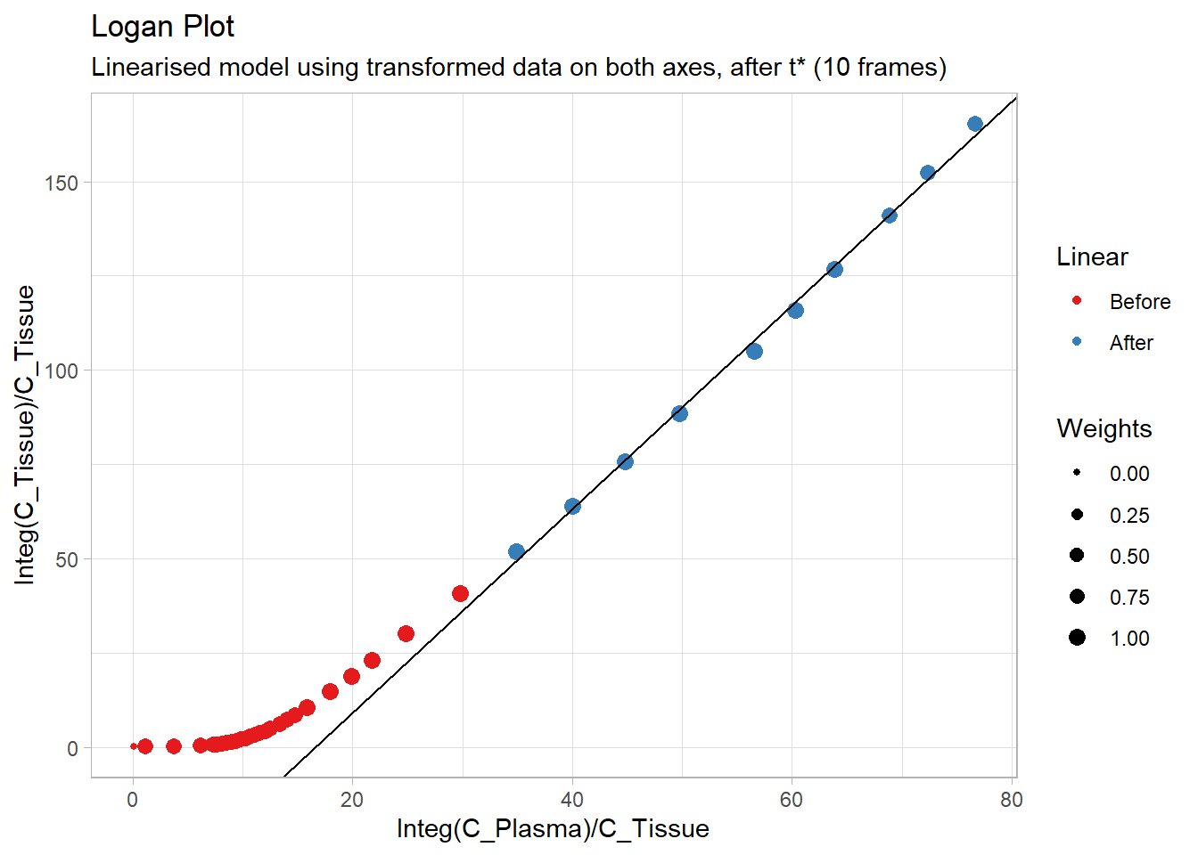
plot(ma1(t_tac, tac, input,
               tstarIncludedFrames =  10,
               weights, inpshift)) +
       labs(title="MA1",
            subtitle="Linearised model predicting actual y values, after t* (10 frames)")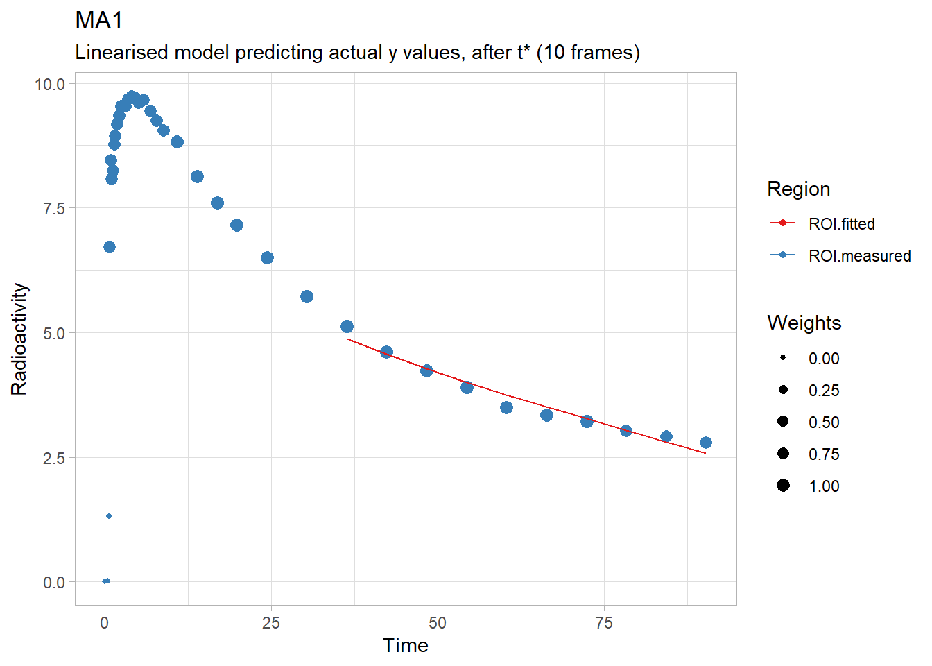
For iteration, where we used the purrr::map and purrr::map2 functions before, we must now use purrr::pmap. This requires us to write a few small functions first. We’ll also just skip returning the whole model fits, and just return the VT values in order to keep this quick and memory usage down. This is mostly for Binder, or those using less powerful machines. I’ll also fit vB using the 2TCM: this is slightly unconventional, but it will make for a good teaching example afterwards.
fit_1tcm <- function(tacdata, input, inpshift) {
  onetcm(t_tac = tacdata$Times/60, tac = tacdata$TAC,
         input = input, weights = tacdata$Weights,
         inpshift = inpshift)$par$Vt
}

fit_2tcm <- function(tacdata, input, inpshift) {
  twotcm(t_tac = tacdata$Times/60, tac = tacdata$TAC,
         input = input, weights = tacdata$Weights,
         inpshift = inpshift)$par$Vt
}

fit_2tcm1k <- function(tacdata, input, inpshift) {
  twotcm1k(t_tac = tacdata$Times/60, tac = tacdata$TAC,
         input = input, weights = tacdata$Weights,
         inpshift = inpshift, vB = 0.05)$par$Vt
}

fit_Logan <- function(tacdata, input, inpshift) {
  Loganplot(t_tac = tacdata$Times/60, tac = tacdata$TAC,
         input = input, weights = tacdata$Weights,
         inpshift = inpshift, vB = 0.05,
         tstarIncludedFrames = 10)$par$Vt
}

fit_mlLogan <- function(tacdata, input, inpshift) {
  mlLoganplot(t_tac = tacdata$Times/60, tac = tacdata$TAC,
         input = input, weights = tacdata$Weights,
         inpshift = inpshift, vB=0.05,
         tstarIncludedFrames = 10)$par$Vt
}

fit_ma1 <- function(tacdata, input, inpshift) {
  ma1(t_tac = tacdata$Times/60, tac = tacdata$TAC,
         input = input, weights = tacdata$Weights,
         inpshift = inpshift, vB = 0.05,
         tstarIncludedFrames = 10)$par$Vt
}

fit_ma2 <- function(tacdata, input, inpshift) {
  ma2(t_tac = tacdata$Times/60, tac = tacdata$TAC,
         input = input, weights = tacdata$Weights,
         inpshift = inpshift, vB=0.05)$par$Vt
}
And now let’s fit the models. We’ll also separate this one out for the purposes of seeing where the boundary limits are hit (the warnings we saw above) (this is why we’re fitting vB, by the way).
pbr28_long <- pbr28_long %>%
  group_by(PET, Region)

  # 1TCM
pbr28_long <- pbr28_long %>%
  mutate("1TCM" = pmap_dbl(list(tacdata, input, inpshift), fit_1tcm))
## Warning: Problem with `mutate()` input `1TCM`.
## i
## Fitted parameters are hitting upper or lower limit bounds. Consider
## either modifying the upper and lower limit boundaries, or else using
## multstart when fitting the model (see the function documentation).
##
## i Input `1TCM` is `pmap_dbl(list(tacdata, input, inpshift), fit_1tcm)`.
## i The error occurred in group 7: PET = "flfp_1", Region = "CBL".## Warning in onetcm(t_tac = tacdata$Times/60, tac = tacdata$TAC, input = input, :
## Fitted parameters are hitting upper or lower limit bounds. Consider
## either modifying the upper and lower limit boundaries, or else using
## multstart when fitting the model (see the function documentation).## Warning: Problem with `mutate()` input `1TCM`.
## i
## Fitted parameters are hitting upper or lower limit bounds. Consider
## either modifying the upper and lower limit boundaries, or else using
## multstart when fitting the model (see the function documentation).
##
## i Input `1TCM` is `pmap_dbl(list(tacdata, input, inpshift), fit_1tcm)`.
## i The error occurred in group 8: PET = "flfp_1", Region = "FC".## Warning in onetcm(t_tac = tacdata$Times/60, tac = tacdata$TAC, input = input, :
## Fitted parameters are hitting upper or lower limit bounds. Consider
## either modifying the upper and lower limit boundaries, or else using
## multstart when fitting the model (see the function documentation).## Warning: Problem with `mutate()` input `1TCM`.
## i
## Fitted parameters are hitting upper or lower limit bounds. Consider
## either modifying the upper and lower limit boundaries, or else using
## multstart when fitting the model (see the function documentation).
##
## i Input `1TCM` is `pmap_dbl(list(tacdata, input, inpshift), fit_1tcm)`.
## i The error occurred in group 9: PET = "flfp_1", Region = "STR".## Warning in onetcm(t_tac = tacdata$Times/60, tac = tacdata$TAC, input = input, :
## Fitted parameters are hitting upper or lower limit bounds. Consider
## either modifying the upper and lower limit boundaries, or else using
## multstart when fitting the model (see the function documentation). # 2TCM
pbr28_long <- pbr28_long %>%
mutate("2TCM" = pmap_dbl(list(tacdata, input, inpshift), fit_2tcm))## Warning: Problem with `mutate()` input `2TCM`.
## i
## Fitted parameters are hitting upper or lower limit bounds. Consider
## either modifying the upper and lower limit boundaries, or else using
## multstart when fitting the model (see the function documentation).
##
## i Input `2TCM` is `pmap_dbl(list(tacdata, input, inpshift), fit_2tcm)`.
## i The error occurred in group 8: PET = "flfp_1", Region = "FC".## Warning in twotcm(t_tac = tacdata$Times/60, tac = tacdata$TAC, input = input, :
## Fitted parameters are hitting upper or lower limit bounds. Consider
## either modifying the upper and lower limit boundaries, or else using
## multstart when fitting the model (see the function documentation).## Warning: Problem with `mutate()` input `2TCM`.
## i
## Fitted parameters are hitting upper or lower limit bounds. Consider
## either modifying the upper and lower limit boundaries, or else using
## multstart when fitting the model (see the function documentation).
##
## i Input `2TCM` is `pmap_dbl(list(tacdata, input, inpshift), fit_2tcm)`.
## i The error occurred in group 9: PET = "flfp_1", Region = "STR".## Warning in twotcm(t_tac = tacdata$Times/60, tac = tacdata$TAC, input = input, :
## Fitted parameters are hitting upper or lower limit bounds. Consider
## either modifying the upper and lower limit boundaries, or else using
## multstart when fitting the model (see the function documentation). # 2TCM1k
pbr28_long <- pbr28_long %>%
mutate("2TCM1k" = pmap_dbl(list(tacdata, input, inpshift), fit_2tcm1k))## Warning: Problem with `mutate()` input `2TCM1k`.
## i
## Fitted parameters are hitting upper or lower limit bounds. Consider
## either modifying the upper and lower limit boundaries, or else using
## multstart when fitting the model (see the function documentation).
##
## i Input `2TCM1k` is `pmap_dbl(list(tacdata, input, inpshift), fit_2tcm1k)`.
## i The error occurred in group 1: PET = "cgyu_1", Region = "CBL".## Warning in twotcm1k(t_tac = tacdata$Times/60, tac = tacdata$TAC, input = input, :
## Fitted parameters are hitting upper or lower limit bounds. Consider
## either modifying the upper and lower limit boundaries, or else using
## multstart when fitting the model (see the function documentation).## Warning: Problem with `mutate()` input `2TCM1k`.
## i
## Fitted parameters are hitting upper or lower limit bounds. Consider
## either modifying the upper and lower limit boundaries, or else using
## multstart when fitting the model (see the function documentation).
##
## i Input `2TCM1k` is `pmap_dbl(list(tacdata, input, inpshift), fit_2tcm1k)`.
## i The error occurred in group 4: PET = "cgyu_2", Region = "CBL".## Warning in twotcm1k(t_tac = tacdata$Times/60, tac = tacdata$TAC, input = input, :
## Fitted parameters are hitting upper or lower limit bounds. Consider
## either modifying the upper and lower limit boundaries, or else using
## multstart when fitting the model (see the function documentation).## Warning: Problem with `mutate()` input `2TCM1k`.
## i
## Fitted parameters are hitting upper or lower limit bounds. Consider
## either modifying the upper and lower limit boundaries, or else using
## multstart when fitting the model (see the function documentation).
##
## i Input `2TCM1k` is `pmap_dbl(list(tacdata, input, inpshift), fit_2tcm1k)`.
## i The error occurred in group 7: PET = "flfp_1", Region = "CBL".## Warning in twotcm1k(t_tac = tacdata$Times/60, tac = tacdata$TAC, input = input, :
## Fitted parameters are hitting upper or lower limit bounds. Consider
## either modifying the upper and lower limit boundaries, or else using
## multstart when fitting the model (see the function documentation).## Warning: Problem with `mutate()` input `2TCM1k`.
## i
## Fitted parameters are hitting upper or lower limit bounds. Consider
## either modifying the upper and lower limit boundaries, or else using
## multstart when fitting the model (see the function documentation).
##
## i Input `2TCM1k` is `pmap_dbl(list(tacdata, input, inpshift), fit_2tcm1k)`.
## i The error occurred in group 8: PET = "flfp_1", Region = "FC".## Warning in twotcm1k(t_tac = tacdata$Times/60, tac = tacdata$TAC, input = input, :
## Fitted parameters are hitting upper or lower limit bounds. Consider
## either modifying the upper and lower limit boundaries, or else using
## multstart when fitting the model (see the function documentation).## Warning: Problem with `mutate()` input `2TCM1k`.
## i
## Fitted parameters are hitting upper or lower limit bounds. Consider
## either modifying the upper and lower limit boundaries, or else using
## multstart when fitting the model (see the function documentation).
##
## i Input `2TCM1k` is `pmap_dbl(list(tacdata, input, inpshift), fit_2tcm1k)`.
## i The error occurred in group 9: PET = "flfp_1", Region = "STR".## Warning in twotcm1k(t_tac = tacdata$Times/60, tac = tacdata$TAC, input = input, :
## Fitted parameters are hitting upper or lower limit bounds. Consider
## either modifying the upper and lower limit boundaries, or else using
## multstart when fitting the model (see the function documentation).## Warning: Problem with `mutate()` input `2TCM1k`.
## i
## Fitted parameters are hitting upper or lower limit bounds. Consider
## either modifying the upper and lower limit boundaries, or else using
## multstart when fitting the model (see the function documentation).
##
## i Input `2TCM1k` is `pmap_dbl(list(tacdata, input, inpshift), fit_2tcm1k)`.
## i The error occurred in group 10: PET = "flfp_2", Region = "CBL".## Warning in twotcm1k(t_tac = tacdata$Times/60, tac = tacdata$TAC, input = input, :
## Fitted parameters are hitting upper or lower limit bounds. Consider
## either modifying the upper and lower limit boundaries, or else using
## multstart when fitting the model (see the function documentation). # Logan
pbr28_long <- pbr28_long %>%
mutate("Logan" = pmap_dbl(list(tacdata, input, inpshift), fit_Logan))
# mlLogan
pbr28_long <- pbr28_long %>%
mutate("mlLogan" = pmap_dbl(list(tacdata, input, inpshift), fit_mlLogan))
# MA1
pbr28_long <- pbr28_long %>%
mutate("MA1" = pmap_dbl(list(tacdata, input, inpshift), fit_ma1))
# MA2
pbr28_long <- pbr28_long %>%
mutate("MA2" = pmap_dbl(list(tacdata, input, inpshift), fit_ma2))
pbr28_long <- pbr28_long %>%
ungroup()We see warnings for some fits of the nonlinear models (these are a bit more verbose in the current version of tidyverse, and helpfully shows which fit had the error, but also shows it twice, which is a bit frustrating). What does this warning mean? Well, when we fit nonlinear least squares models, we provide starting values, as well as upper and lower limits for each of the parameters, and then our model hops around parameter space using gradient descent to try to find the parameters which maximise the likelihood of the data (i.e. they move around parameter space until they find a set of parameters which, moving in any direction causes the fit to worsen). This does not guarantee that we find the best set of parameters: there are potentially a multitude of local minima (places where the cost function is low relative to surroundings), but these can be different from the global minimum (the best possible set of parameters). This warning emerges because we’ve landed up against one of our limits in one of our parameters. This could either be due to having set upper and lower values which are too restrictive, or it could be because our model is landing in a local minimum, or chasing the parameters off into a corner: our model can compensate for bad estimates in one parameter by adjusting one of the other parameters. This is almost the definition of poor identifiability: the noise in the data is such that the model cannot identify a unique set of parameters which describes it best: rather there are numerous combinations of the parameters which all describe the (noisy) data about as well as each other. Conveniently, however, most of these sets of parameters result in similar VT estimates.
Anyhow, to solve this, we could either mess about with the starting parameters, the upper limits or the lower limits. Otherwise, if we think that the limits are ok, and the fit is just going in the wrong direction, we can set the model to fit multiple times using a bunch of different starting parameters and choose the best fit, using the nls.multstart package. Let’s try for one fit. The seventh fit was one such failure (so, to be fair, setting vB did prevent this for this particular TAC. But I’ll fit vB here just to demonstrate the point).
i=7
tacdata = pbr28_long$tacdata[[i]]
input = pbr28_long$input[[i]]
inpshift =  pbr28_long$inpshift[i]

badfit <- twotcm(t_tac = tacdata$Times/60, tac = tacdata$TAC,
                  input = input, weights = tacdata$Weights,
                  inpshift = inpshift)
## Warning in twotcm(t_tac = tacdata$Times/60, tac = tacdata$TAC, input = input, :
## Fitted parameters are hitting upper or lower limit bounds. Consider
## either modifying the upper and lower limit boundaries, or else using
## multstart when fitting the model (see the function documentation).badfit$par## K1 k2 k3 k4 vB inpshift Vt
## 1 0.2285033 0.06959382 0.5 0.5 0.08756467 0.04581712 6.566769Now, those k3 and k4 values look extremely high: they mean that 50% of what’s in the non-displaceable compartment is entering the specific compartment every minute, and 50% of what’s in the specific compartment is entering the non-displaceable compartment each minute. This is essentially fitting a one-tissue compartment model, as it’s assuming that the equilibrium between these two compartments is so rapid. We know, from the rest of the sample, and from previous experience with this tracer, and other studies using this tracer, that that doesn’t sound quite right. So let’s try with multstart. We can either provide a single value (for which it just chooses that number of randomly selected starting parameters from across parameter space and fits the model), or we can even provide a vector of numbers, which defines an grid across each of the parameters fitted in the model and tries at each point. Because we’re being lazy, let’s just use the former, simpler approach (the latter is really a nuclear option…)! Note: always good to set a seed with multstart, as it samples randomly. So it’s worth being very particular about this to be sure that it works.
set.seed(42)
multstartfit <- twotcm(t_tac = tacdata$Times/60, tac = tacdata$TAC,
                        input = input, weights = tacdata$Weights,
                        inpshift = inpshift,
                        multstart_iter = 20)
And, no warnings! Let’s check those parameters compared with the old ones.
bind_rows(badfit$par, multstartfit$par) %>%
  mutate_all(~round(.x, 3)) %>%
  mutate(Method=c("Single Fit", "Multstart Fit"))
## K1 k2 k3 k4 vB inpshift Vt Method
## 1 0.229 0.070 0.500 0.500 0.088 0.046 6.567 Single Fit
## 2 0.254 0.075 0.043 0.035 0.074 0.046 7.525 Multstart FitWe can see that our VT values were somewhat consistent (though actually, this is an uncharacteristically large deviation). But we can also see that k3 and k4 have changed a great deal. We could probably have resolved this from the start by setting better starting parameters, as the defaults are 0.1 and 0.1 respectively.
Just a note: the reason this is happening is more a product of PBR28 as a radiotracer than anything else. It isn’t quite fit correctly even by the 2TCM, and it’s generally a bit of a nightmare for modellers (I personally trust MA1 much more for this tracer). Using multstart, in addition to being a bit slower, also adds a little bit of extra randomness to the equation. But it can also be a lifesaver when things are acting up.