TOC
Introduction
I wanted to do something different on this blog and go through something that’s less of my side-project, and more of my project project, i.e. PET pharmacokinetic modelling. I’ll discuss a little bit of the theory, and then I’ll go through practical implementation of these models using my R package kinfitr in a series of blog posts. Here, in part 1, I’ll go through some of the theory.
The parts of this series are as follows:
A Whirlwind guide to PET Modelling
First, I wanted to go into a bit of the theory of PET for anyone who is interested. I hope the problems themselves are as interesting to others as they are to me. These models tend to fit the data very cleanly (often), with models that are theoretically-grounded in the biological considerations and constraints. Furthermore, the outcome parameters are almost all grounded in actual SI units.
Firstly, what is Positron Emission Tomography (PET)? PET is a method for quantification of proteins or metabolic processes in the body. We use one of a variety of ligands which bind to the thing we’re interested in (the target molecule), and we replace one of the ligand’s atoms with a radioactive isotope to form a radiotracer. Then, we inject it into the blood, and we observe the subsequent changes in radioactivity concentrations with time. Using a PET camera, we can measure radioactivity at high spatial resolution (<5mm). Using this method, we typically assess proxies of the concentrations of certain proteins (e.g. do X patients have more of Y receptor in Z region of the body), or assess the extent to which another compound (either a pharmacological compound or a chemical originating from the body) occupies the same binding site and displaces our radioligand.
In order to get an idea of the dynamics of the radioactivity concentrations, we divide our image up into a number of frames, reconstruct the observed radioactivity into images (leaving us with a series of 3D images) (this step involves some really neat physics for those of you who are interested, but irrelevant for this summary). Using an anatomical MR image, we spatially register the two images together, and take the mean radioactivity within a given region for each frame, resulting in what is called a time-activity curve (TAC).
While classic pharmacokinetic modelling aims is usually concerned with estimating the concentration of a drug in the body at various time points, in PET we are usually more interested in assessing the concentration of the target molecule in a given part of the body. Another main difference is that in classic pharmacokinetic modelling, you are usually interested in the concentration of the ligand in the blood where it was injected, while in PET we are typically interested in a specific area of the body (in my case, usually different regions of the brain). What this means is that we deliver the radioligand to the blood, and the blood delivers the ligand to the brain, and we need to account for this gradual delivery.
Compartmental Modelling
At the heart of most of our kinetic models, we have compartmental models. We draw boxes with arrows describing the rate of transfer between these boxes, and then we estimate the rates of transfer and the concentrations within each of our boxes. A simple example is the one-compartment model: we have radiotracer originating in the blood (C_0_), and crossing the blood-brain barrier at a certain rate (K1), and then we have the same compound crossing the blood brain barrier at another rate (k2) as it leaves the brain again. This tracer would be called reversible, in that it enters the compartment, and then leaves the compartment. If k2 were to be equal to 0, it would be irreversible.
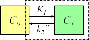
One-Tissue Compartment Model: Image from http://www.turkupetcentre.net/petanalysis/model_compartmental.html
A two-compartmental model then consists of another compartment after the first, which receives radiotracer from the first compartment. Thus, we add the rate constants k3, the travel of radiotracer from the first to the second compartment, and k4, its reverse. As above, if k4 were to be equal to 0, the binding to the second compartment would be irreversible.
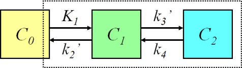
Two-Tissue Compartment Model: Image from http://www.turkupetcentre.net/petanalysis/model_compartmental.html
Most models, in biological terms, originate from the three-tissue compartment model, with compartments representing specifically-bound radiotracer (i.e. the stuff we’re interested in), non-specifically-bound radiotracer (i.e. the stuff we’re not interested in), and the free radiotracer (i.e. that is capable of going into one of the other two compartments, or into the blood). This model is very complex, and has a lot of parameters, and I’ve never seen it used in practice. We usually collapse compartments together under the assumption that transfer between them is so rapid as to render the two compartments in constant equilibrium. So, to get the classic two-compartment model, we collapse the free and non-specifically bound compound into a compartment called the non-displaceable compartment (i.e. stuff that another compound that binds to the target molecule wouldn’t displace). And these two are collapsed into one another for the one-compartment model, if dynamics are very fast between all three compartments. Fewer compartments means fewer parameters to fit, which usually means more robust estimates which fit faster. However, if we underfit the data too badly, we can get severely biased estimates.
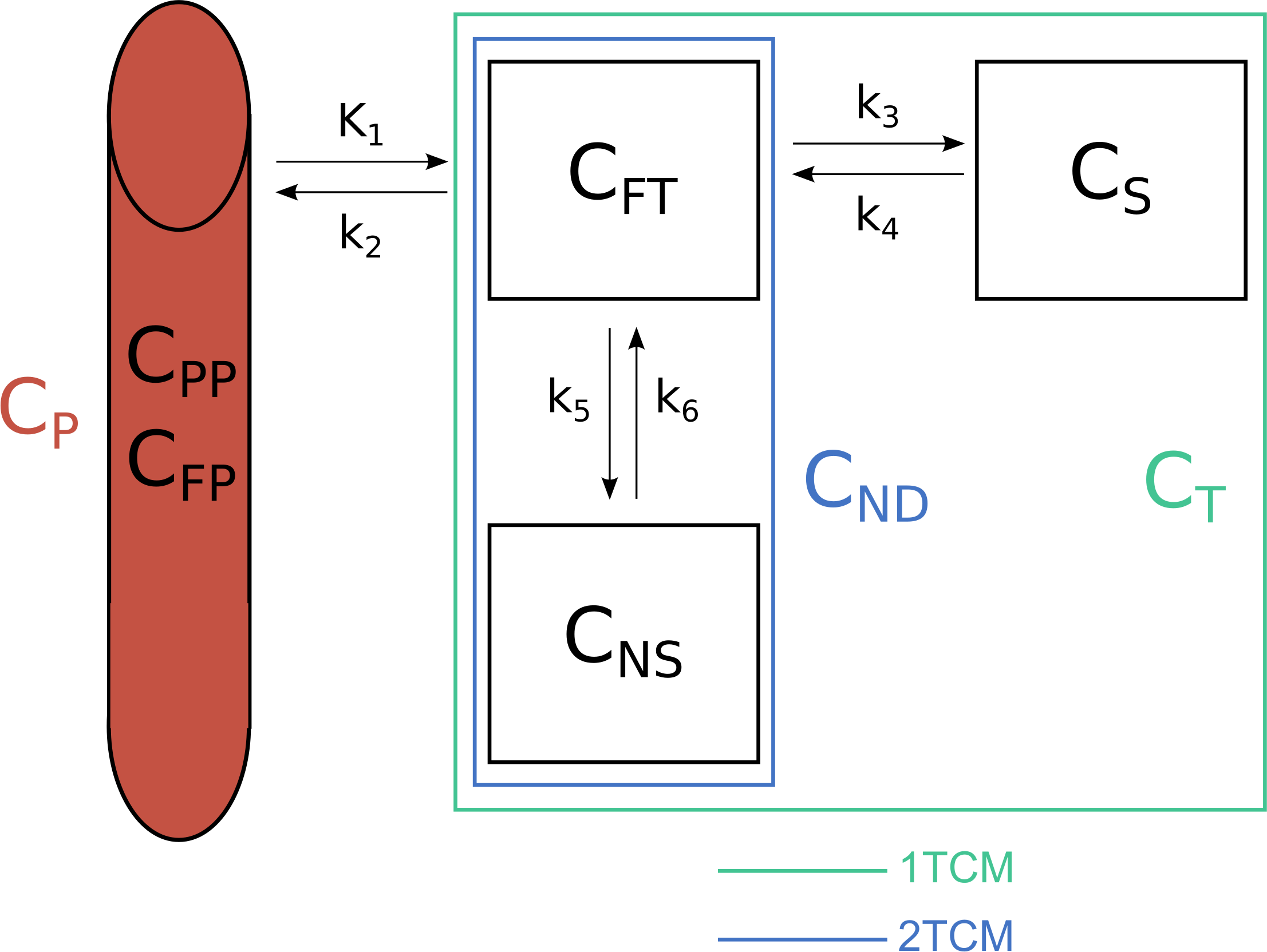
The three-tissue compartment model, and the compartments which are joined to create the two-tissue compartment model, and the one-tissue compartment model.
Importantly, all of these models require us to know about what’s going on in the blood to know about the delivery to the brain. This poses a host of difficulties of its own (discussed below). Another method to quantify our signal is to use a reference region: this is another region of the body/brain which has none, or at least negligible quantities of specific binding. In this way, by comparing the two regions, one with and one without specific binding, and assuming that the two have equal non-displaceable binding, we can estimate the specific binding.
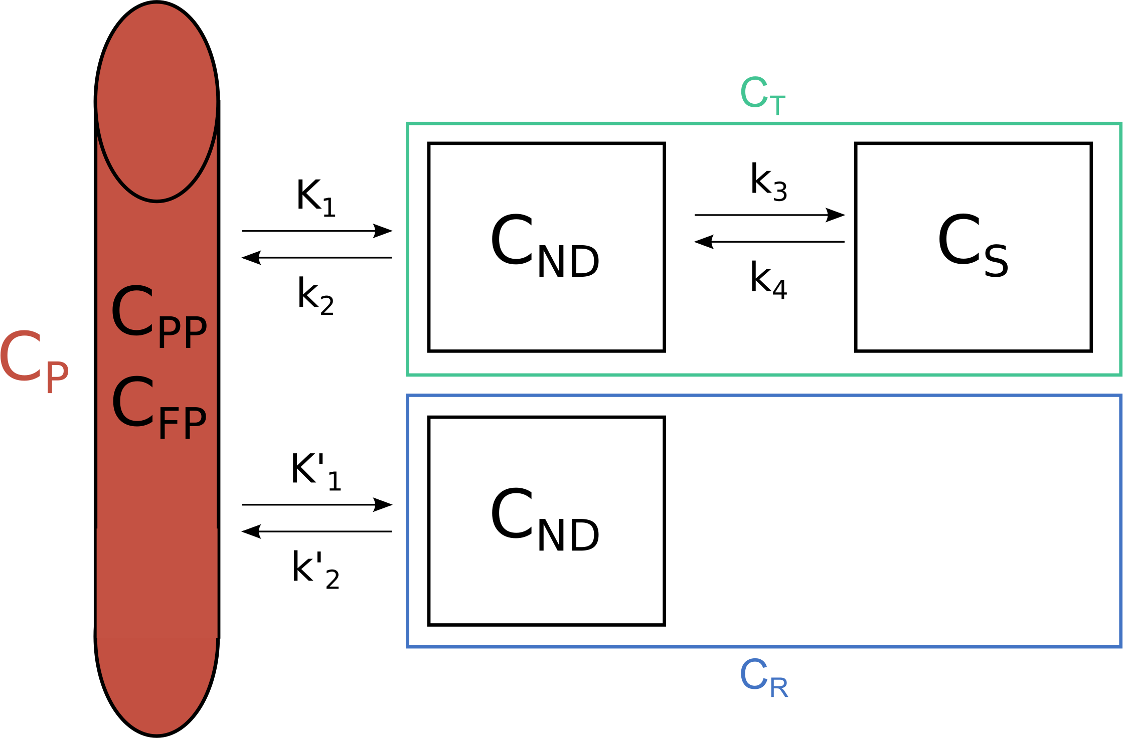
Reference tissue models are based on the assumption of equal non-displaceable binding in target and reference regions.
What we do with Blood, and Why it’s Hard
Having discussed the models above and their relation to the concentration of the radiotracer in blood, we obviously need to actually know the concentration in the blood. We do this by taking a series of measurements of blood radioactivity. The dynamics in the blood are very fast though, and so we need to take a lot of measurements, and sometimes we also use an automatic sampler too.
We can think of the blood as a series of deliveries of the radiotracer into the brain of varying size. A good analogy by a colleague (Martin Schain), is that we can think of each delivery like pouring a bucket of water into a bath, which then flows out through the plughole. If we were just interested in the concentration following a single dose, we would dump it in and watch it flow out gradually through the plug hole. Instead we dump in a small bucket of water, and then, before it has run out, we dump in the next slightly-larger bucket etc etc.
Mathematically, this is instantiated by a convolution (\(\otimes\)) between the blood curve (AIF) and an impulse response function (IRF). The impulse response function is the expected curve if we could perform the perfect instantaneous injection of the radiotracer to the region itself: it would be the equivalent of pouring one single bucket of water into the bath, and is described by an exponential decay, or a sum of exponential decays.
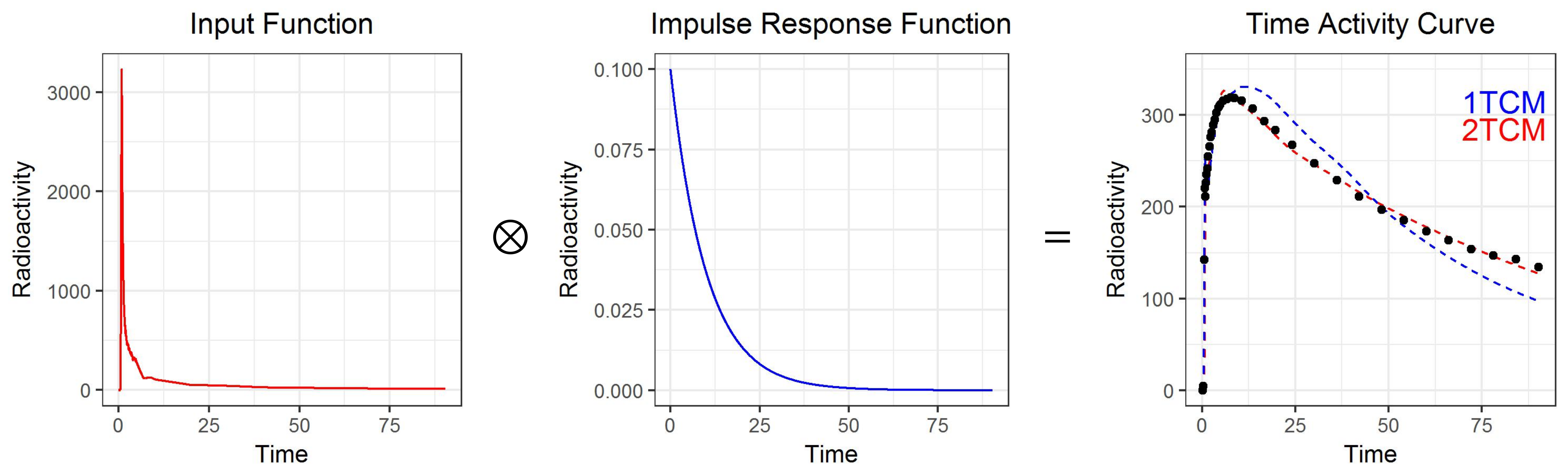
The arterial input function (AIF, left, measured) is convolved with the impulse response function (IRF, centre, fitted), to produce the time activity curve (TAC, right, measured).
The calculation of the convolution can be thought of as reversing one of the curves, and then sliding them through one another. The resulting, convolved, function at each time point is equal to the overlapping area of the two curves.
So, if we could inject a perfect instantaneous bolus, we would observe the IRF, and the shared area is just equal to the height of the IRF at each time point.
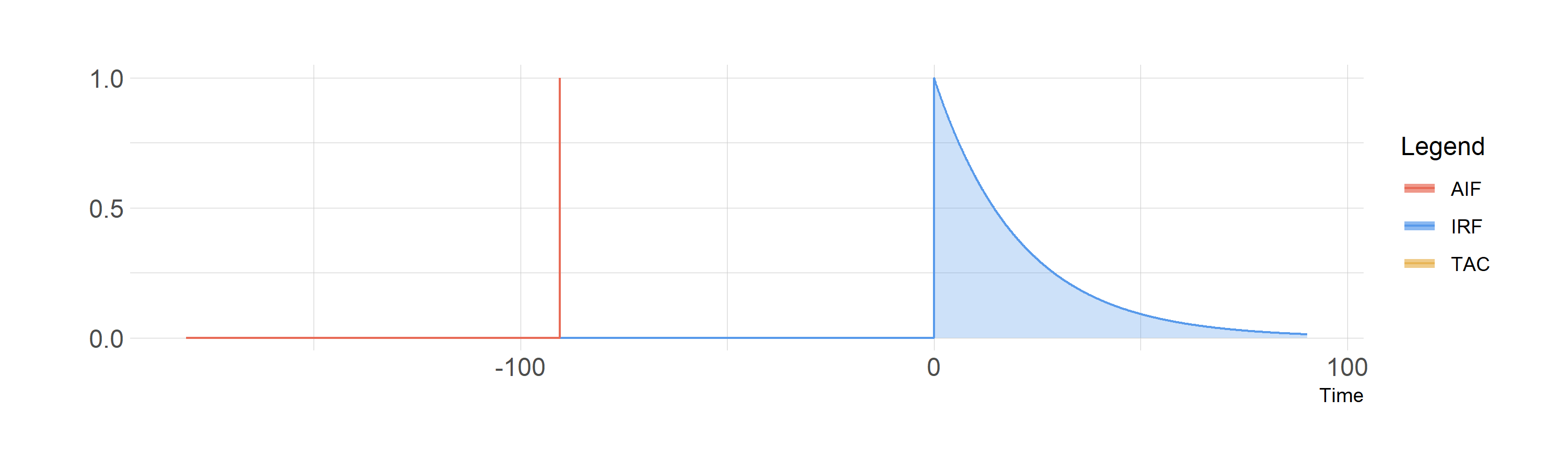
Convolution of a perfect bolus with the IRF
And below we see the convolution of the AIF with the IRF, with the shared area depicted in the same colour as the TAC. Note that I’ve scaled all three curves to be the same height, which is not the case: the AIF is much higher than the TAC - but this would make it much more difficult to see what was going on.
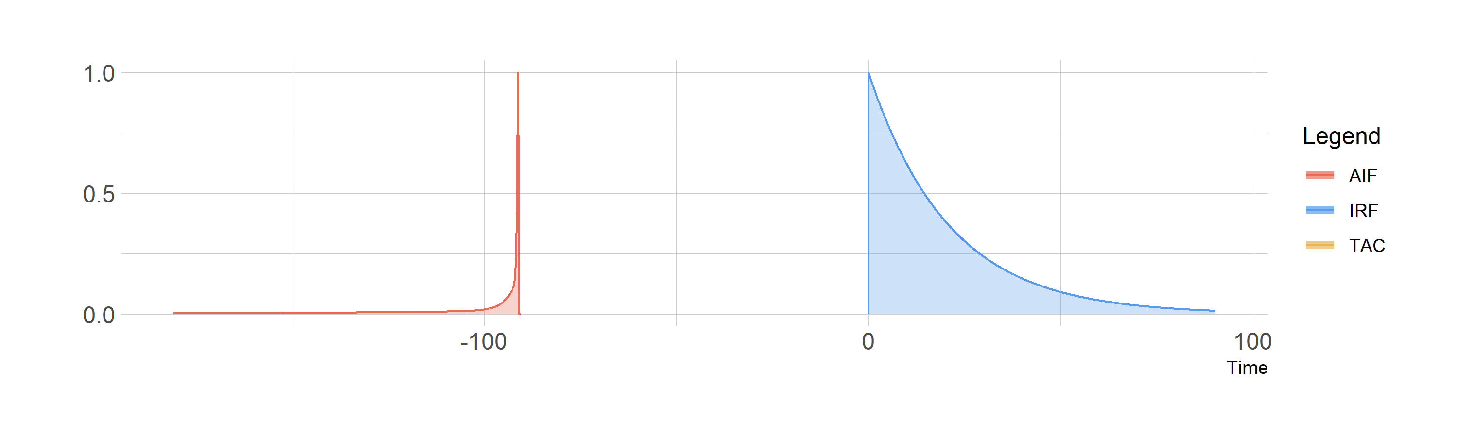
Convolution of the blood curve (AIF) with the IRF
But what makes the measurement of the blood curve, the AIF, so hard? Well, actually, a number of things.
We can’t just collect any blood: we need to collect arterial blood (i.e. from an artery, not a vein) because this is the blood being pumped out from the heart to different parts of the body. Arterial blood gives us a good approximation of the concentration of the tracer in the blood heading for the brain, but it involves specialised staff to insert the needle.
We’re not actually particularly interested in the blood: the radioactivity that enters the brain is in the blood plasma. So we need to remove the red blood cells from the blood to get an idea of the radioactivity in the arterial blood plasma. In some of our manual samples, we will measure both blood and plasma so that we can calculate the blood-to-plasma ratio, interpolate this curve and estimate plasma concentrations from all blood measurements.
Over time, our compound is also metabolised by the body, so that it no longer enters the brain (hopefully - usually). But the radioactivity is still there. So we also put a bunch of our plasma samples into an HPLC (a big chemistry machine) to estimate the proportion of the radioactivity that is attributable to the original compound, i.e. the parent fraction in the arterial blood plasma. We need to interpolate this curve too to multiply all plasma radioactivity concentrations by to get the metabolite-corrected arterial plasma concentration.
Bear in mind too that the dynamics are very quick. So there are several people involved, taking blood samples, recording when they were taken, and operating all the machines to analyse the samples as they are taken (because the radioactivity concentrations are constantly decreasing too).
So, basically, taking these samples is unpleasant for participants because they come from the artery, and to get a good idea of the blood curve that we use for the modelling, we need to interpolate (or model) the parent fraction measurements and the plasma radioactivity measurements, as multiplicative correction factors for the blood radioactivity measurements; all of which are measured with some degree of error. The resulting curve is called the metabolite-corrected arterial input function, or AIF for short.
As a result, it’s really preferable to be able to find a reference region in the brain: it’s not only cheaper and easier, but also tends to be less error-prone. But when there just simply isn’t any region of the brain without the target molecule, then we often have to use these models with arterial blood.
Models and Outcome Parameters: Why So Many?
When it comes to quantification, we have to make compromises to get what we want as well as we possibly can. This is one of, if not the central consideration when performing PET modelling. We must consider the data that we have, our research question, the radioligand in question etc to find the compromise that works best for our purposes. We are often forced to make assumptions which are not strictly true in order to estimate a quantity in a manner which is slightly wrong as a result, but wrong in a way that we hope shouldn’t affect our conclusions in too drastic a manner, based on what we are specifically interested in. I think there’s a lot of fun to be had in this domain as a modeller, and this is one of the primary motivations for the creation of the kinfitr package.
Outcome parameters
There are two primary classes of outcome measures: volumes of distribution (V), and binding potential (BP). Both relate radioactivity in various compartments with other compartments. In each case, when I talk about the “amount of radioactivity”, I refer to the integral of the impulse response curve (i.e. an instantaneous influx of an amount of 1, and its gradual efflux). This can also be conceptualised as the integral of the measured curve divided by the integral of the input curve, since we consider the input to be a series of micro-influxes, and the resulting measured curve to be the result of multiple overlapping effluxes.
Volumes of distribution compare the quantity of the radioligand in the target tissue to the amount of times the blood containing the radioligand would need to be in that compartment. We can consider several different compartments: VT is the total distribution volume (i.e. in all compartments of the target tissue), VND is the distribution in the non-displaceable compartment, and VS is the distribution volume in the specific compartment.
Consider a VT of 1: this means that, at equilibrium, the amount of radioactivity in the blood and the amount of radioactivity in the target tissue would be equal. Consider the 1-tissue compartment model: that would mean that the influx (K1) would be equal to the efflux (k2). Thus, the volume of distribution is equal to \(\frac{K_1}{k_2}\).
Binding potential on the other hand compares the quantity of the radioligand in the specific compartment to other compartments. Specific binding can be compared to blood plasma (BPP), to non-displaceable binding (BPND). If you’re attentive, you’ll notice that BPP is the same thing as VS.
For those who are interested, each of these quantities can also be described by combining the rate parameters.
In the 1TCM, there is only one compartment, so it’s only possible to estimate VT.
- \(V_T=\frac{K_1}{k_2}\).
For the 2TCM, we can do more.
\(V_T=\frac{K_1}{k_2}(1 + \frac{k_3}{k_4})\)
\(V_{ND}=\frac{K_1}{k_2}\)
\(V_S=BP_P=\frac{K_1k_3}{k_2k_4}=V_T-V_{ND}\)
\(BP_{ND}=\frac{k_3}{k_4} = \frac{V_S}{V_{ND}}\).
Not that there are also some additional outcome parameters for irreversibly-binding radioligands, but I’ll not go into those here, as most modelling applications are interested in reversibly binding ligands.
Importantly, you will need blood data to estimate distribution volumes. BPND, on the other hand, is usually estimated by reference region models. Using blood data, however, the most common outcome parameter is VT, rather than VS. This seems paradoxical: VT contains non-displaceable binding too, which gets in the way of the actual thing we’re interested in, i.e. specific binding. However, VT is usually estimated with much greater precision that VS. In cases of estimating BPND or VT, and comparing individuals using these outcomes, we typically make the assumption that VND is equal between individuals and regions though, which may be more or less true depending on the specific radioligand. This is a example of one of the compromises I mentioned above.
Models
When it comes to models, we have a great many, which ideally all converge to nearly identical answers, but not always. While all models using blood are essentially based on the three-tissue compartment model, all models using reference tissues are essentially based on the full reference tissue model. And neither of these are used in regular practice. Rather, much of the work which has gone into modelling PET has focused on smart ways to reduce the number of parameters using clever assumptions. Nonlinear least squares fitting is used to model many models within PET: the classic 1, 2 and 3 compartment models, as well as full (and simplified) reference tissue models, among others. However, there are also a number of linearisations of these models using asymptotic approximations.
The linearisations are obviously quicker, and tend to be quite robust, but there is also an element of bias for many applications: sometimes more noise systematically biases binding estimates due to correlated errors in the dependent and independent variables. Additionally, most of the linearisations can only examine the total binding (VT for blood models, and BPND for reference-tissue models). If we were to be specifically interested in the rate constants or in one compartment in particular, these models do not give us this information. Additionally, with nonlinear models, one can set upper, lower and starting values for the parameters in order to most appropriately constrain our model: these can be used to constrain our model to reasonable parameters (and, yes, Bayesian priors and a multilevel framework would be awesome here: that’s my postdoc project). There are also models for irreversibly-binding tracers, but I don’t deal with these much.
In short, it’s good to have a big toolbox at hand when modelling especially a new tracer, but even established tracers depending on specific research questions, or if the data is especially clean or noisy. With flexibility, it also become extremely important to be able to be transparent about exactly what you have done, and to work reproducibly.
…and that’s where my kinfitr package comes along!
I hope you’ve enjoyed the theory: I think it’s a really nice problem-space, and the models themselves and their derivations are really elegant. If you want to read more, I can refer you to the introduction of my thesis, the Turku PET Centre guide, or to one of many books or articles about PET modelling (Turku has a great list of good resources here). Now let’s dive into how we might perform a basic analysis in the following parts of this tutorial.